Wichita, Kansas

Weather Forecast Office

Assessment of NCEP and Local Area Model Forecasts of Convection and Reflectivity

Assessment of NCEP and Local Area Model Forecasts of Convection and Reflectivity

Kenneth R. Cook, Jacob R. Wallentine, and Kevin R. Rider
National Weather Service, Wichita, Kansas

March 24th, 2010

1.0 Introduction

Convective forecasts are of great importance to those on the Plains due to the severity and frequency of occurrence in this region of the country. Many forecasters use NWP (Numerical Weather Prediction) in conjunction with observational data sets to assess the environment. This is done to ascertain the mode of convection that will occur as well as the time in which it will initiate. As NWP has progressed over the years, fields can now be produced to replicate the reflectivity of radar echoes, giving forecasters a first hand look at modeled storm mode outcomes. Additionally, higher temporal resolution from NWP may give forecasters a leg up in preparing for a high impact events should the beginning and evolution be better depicted.

This study was launched to better ascertain the performance of local and national models with regards to convective initiation (CI) and reflectivity performance. This should give forecasters data that will enable them to better understand the advantages and limitations of both NCEP and Local Area Model (LAM) models.

2.0 Methodology

2.1 Model's Used

Cases were selected from the study domain, which for this study included Kansas and Oklahoma. In Oklahoma, the study area was limited to the region north of I-40. Convection had to initiate in this area. This afforded the inclusion of 2 LAM runs, both using WRF-ARW cores and the Local Analysis and Prediction System (LAPS) initialization. Some additional configuration information on the LAMs:

Information	WRFARW16	WRFARW32
Horizontal Resolution	16 km	32 km
Vertical Levels	51	51
Time Steps	1 hour	3 hour
Initialization	LAPS	LAPS
LBC	NAM-WRF	GFS
CP Scheme	KF	KF

A total of 43 cases were examined. NWP models used in this part of the study:

Model	Description
NAM-WRF	12km WRF produced by NCEP
RUC40	40km RUC produced by NCEP
WRFARW16	16km LAM (see above)
WRFARW32	32km LAM (see above)
WESTNMM4	4km SPC WRF NMM Core for Western U.S.
WESTARW4	4km SPC WRF ARW Core for Western U.S.
EASTNMM4	4km SPC WRF NMM Core for Eastern U.S.
EASTARW4	4km SPC WRF ARW Core for Eastern U.S.

All of these models have a maximum of a 3 hour time-step. For the second part of this study, which involved only models that produced reflectivity output, the NAM-WRF and the RUC40 were excluded.

2.2 CI Location and Time

CI was identified as first echo on the WSR-88D and was compared to the location of first model QPF accumulation that was deemed associated with CI. A CI location error was determined by finding the distance between these two features. The time error was found by identifying the hour that first echo was observed, rounded to the next hour. Thus making it consistent with the way in which model QPF is accumulated. The data was then placed into a scoring system to better determine the overall performance.

2.3 Reflectivity Evolution and Performance

A subjective assessment was made (1-5, 5 being the best) on NWPs prediction of the system evolution as represented by the reflectivity output. A further determination was made, using the same scale, on the performance of the reflectivity data. To better understand these, the system evolution would characterize the storm mode and any evolutionary processes (e.g. Supercell to QLCS) that took place. The performance was based on the location, speed, and representation of the radar observed reflectivity. It should be noted that the same individual assessed either the evolution or performance to reduce any biases that could have been included in the data. The data was then placed into a scoring system to better determine the overall performance.

3.0 Analysis and Results

3.1 Convective Initiation

3.1.1 Location

CI location errors were computed using 25 mile increment range bins. For example, if an error of 37 miles was observed from the point of CI, it fell into the 50 mile range bin. These results can be seen in table 1 and are plotted in figure 1. From the results, we then scored each based on skill, multiplying a skill category error (1-5, 5 being the least error/most skill) by the number of occurrences in each category. From these resultant calculations, we were able to find where each model fell within the skill categories.

Results are shown in table 2. The top 2 are highlighted. From these data, the NAM-WRF40 and the RUC40 were the best predictors, with an average skill category of just over 4, meaning the average error was between 25 and 50 miles.

Model	25 miles	50 miles	75 miles	100 mi	150 mi	150 mi +	Total
WRFARW32	21	7	6	3	6	0	43
NAM40	22	9	8	0	4	0	43
WESTNMM4	14	9	3	5	5	0	36
WESTARW4	15	9	0	4	5	0	33
EASTNMM4	18	8	8	3	1	2	40
EASTARW4	12	6	5	5	1	2	31
RUC40	25	4	7	2	3	0	41
WRFARW16	17	13	5	2	4	0	41

Table 1. Number of occurrences of model in each distance error bin.

Fig. 1. Spatial error of the convective initiation location.

Model	5	4	3	2	1	Total	Average
WRFARW32	105	28	18	6	6	169	3.79
NAM40	110	36	24	0	4	174	4.05
WESTNMM4	70	36	9	10	5	130	3.61
WESTARW4	75	36	0	8	5	124	3.76
EASTNMM4	90	32	24	6	1	153	3.83
EASTARW4	60	24	15	10	1	110	3.55
RUC40	125	16	21	4	3	169	4.12
WRFARW16	85	52	15	4	4	160	3.90

Table 2. Number of points of model in each distance error bin. Also shows the total and average number of points for each model.

3.1.2 Time

CI time errors were computed using 1 hour increment bins. The results can be seen in table 3 and are plotted in figure 2. From the results, we then scored each based on skill, multiplying a skill category error (1-5, 5 being the least error/most skill) by the number of occurrences in each category. From these resultant calculations, we were able to find where each model fell within the skill categories.

Results are shown in table 4. The top 2 are highlighted. From these data, the local WRFARW16 and the RUC40 were the best predictors, with an average skill category of near 4, meaning the average error was around 2 hours.

Model	1 hour	2 hours	3 hours	4 hours	6 hours	6 hours +	Total
WRFARW32	15	10	5	7	3	2	42
NAM40	12	10	10	5	4	1	42
WESTNMM4	5	10	5	7	4	5	36
WESTARW4	2	9	5	5	5	7	33
EASTNMM4	5	10	9	8	7	2	41
EASTARW4	5	7	7	6	4	3	32
RUC40	15	15	7	1	0	1	41
WRFARW16	16	14	7	3	1	1	42

Table 3. Number of occurrences of model in each hour error bin.

Fig. 2. Temporal error of the convective initiation time.

Model	25 miles	50 miles	75 miles	100 mi	150 mi	Total	Average
WRFARW32	75	40	15	14	3	147	3.50
NAM40	60	40	30	10	4	144	3.43
WESTNMM4	25	40	15	14	4	98	2.72
WESTARW4	10	40	15	10	5	76	2.30
EASTNMM4	25	40	27	16	7	115	2.80
EASTARW4	25	28	21	12	4	90	2.81
RUC40	75	60	27	2	0	164	4.00
WRFARW16	80	56	21	6	1	164	3.90

Table 4. Number of points of model in each error bin. Also shows the total and average number of points for each model.

3.1.3 Final Assessment

To ascertain which model performed best in this portion of the study, the two skill scores were averaged. The results are found in table 5, showing the RUC40 and the WRFARW16 being the best overall performers. A clear demarcation was noted in these performers and are highlighted in table 5. These show that LAMs do provide some local skill and can improve on the forecast if used and configured optimally.

Model	Overall Avg.
WRFARW32	3.65
NAM40	3.74
WESTNMM4	3.17
WESTARW4	3.03
EASTNMM4	3.31
EASTARW4	3.18
RUC40	4.06
WRFARW16	3.90

Table 5. Number of points, implying the total combined performance

3.2 Reflectivity

3.2.1 Evolution

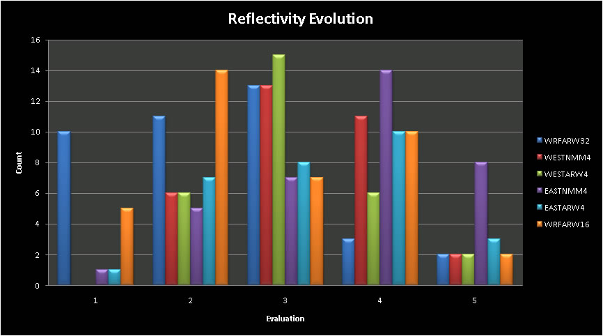
Reflectivity evolution was subjectively scored according to skill. This "skill" ascertained the ability of NWP to properly indicate storm mode and system evolution to an alternate storm mode if applicable. Table 6 and figure 3 both show the scores, where the higher number indicates more skill or better depiction of storm mode and evolution. From the results, we then scored each based on skill, multiplying a skill category error (1-5, 5 being the most skill) by the number of occurrences in each category. From these resultant calculations, we were able to find where each model fell within the skill categories.

Results are shown in table 7 below. The top 2 are highlighted. From these data, both the SPC NMM cores outperformed the remainder of the models. This may be due to more vertical levels within the model as they are currently configured and run. The ARW cores are currently running with a reduction in the vertical levels in order to get the run completed in a timely fashion to fit into the NCEP modeling schedule.

Model	1	2	3	4	5	Total
EASTARW4	1	7	8	10	3	29
EASTNMM4	1	5	7	14	8	35
WESTARW4	0	6	15	6	2	29
WESTNMM4	0	6	13	11	2	32
WRFARW16	5	14	7	10	2	38
WRFARW32	10	11	13	3	2	39

Table 6. Number of occurrences of model in each evolution bin.

Fig 3. Character of reflectivity evolution .

Model	1	2	3	4	5	Total	Average
EASTARW4	1	14	24	40	15	94	3.24
EASTNMM4	1	10	21	56	40	128	3.66
WESTARW4	0	12	45	24	10	91	3.14
WESTNMM4	0	12	39	44	10	105	3.28
WRFARW16	5	28	21	40	10	104	2.74
WRFARW32	10	22	39	12	10	93	2.38

Table 7. Number of points of model in each evolution bin. Also shows the total and average number of points for each model.

3.2.2 Performance

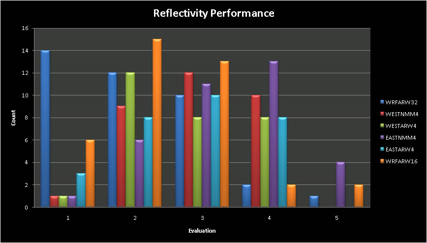
Reflectivity performance was subjectively scored according to skill. This "skill" ascertained the ability of NWP to properly indicate a location, speed, and representation of the radar observed reflectivity. Table 8 and figure 4 both show the scores, where the higher number indicates more skill or better performance of the model forecast radar reflectivity. From the results, we then scored each based on skill, multiplying a skill category error (1-5, 5 being the most skill) by the number of occurrences in each category. From these resultant calculations, we were able to find where each model fell within the skill categories.

Results are shown in table 9 below. The top 2 are highlighted. From these data, both the SPC NMM cores again outperformed the remainder of the models, likely for the same reason indicated in the previous section.

Model	1	2	3	4	5	Total
EASTARW4	3	8	10	8	0	29
EASTNMM4	1	6	11	13	4	35
WESTARW4	1	12	8	8	0	29
WESTNMM4	1	9	12	10	0	32
WRFARW16	6	15	13	2	2	38
WRFARW32	14	12	10	2	1	39

Table 8. Number of occurrences of model in each performance bin.

Fig 4. Character of reflectivity performance.

Model	1	2	3	4	5	Total	Average
EASTARW4	3	16	30	32	0	81	2.79
EASTNMM4	1	12	33	52	20	118	3.37
WESTARW4	1	24	24	32	0	81	2.79
WESTNMM4	1	18	36	40	0	95	2.97
WRFARW16	6	30	39	8	10	93	2.45
WRFARW32	14	24	30	8	5	81	2.08

Table 9. Number of points of model in each evolution bin. Also shows the total and average number of points for each model.

3.2.3 Final Assessment

When comparing these data averages, table 10 indicates the best in the reflectivity category, the SPC NMM cores.

Model	Overall Avg.
EASTARW4	3.02
EASTNMM4	3.51
WESTARW4	2.97
WESTNMM4	3.13
WRFARW16	2.59
WRFARW32	2.23

4. Overall Conclusions

Using NWP in the forecast process to forecast CI and solutions can be difficult. That said, current advancements in technology have afforded us the ability to view a model forecast of radar reflectivity. One can infer from these data storm modes, movement, and evolution. The goal of this project was to give the forecaster a better understanding as to the performance of NWP for convection in the the proximity of the National Weather Service's Wichita County Warning Area.

The results showed that for CI location and time, the NAM40, RUC40, and the 2 LAMs were the best performers with a clear demarcation in performance skill scores. Regarding the performance and evolution of the reflectivity data, the two 4km SPC WRFNMM cores outperformed the remainder of the models.