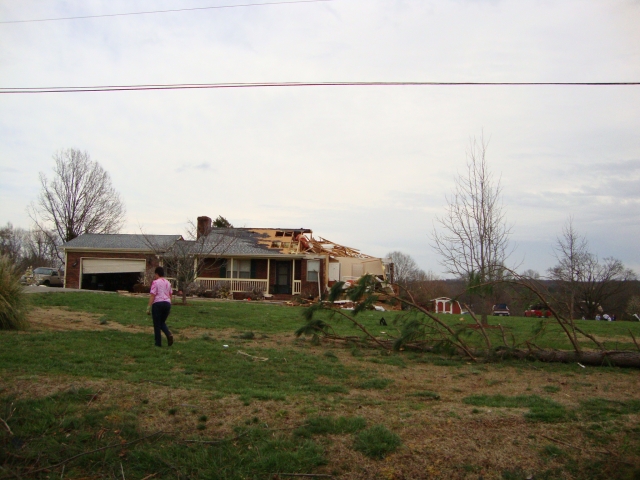
Damage to single family wood frame houses on Brookstead Meadow Court in eastern Mecklenburg County from the Harrisburg Tornado on 3 March 2012. The vantage point is approximately the direction from which the tornado came. Note the convergent pattern of the damage to the houses on the far left and far right. Image obtained from The Charlotte Observer and used by permission.

Author's Note: The following report has not been subjected to the scientific peer review process.

1.  Introduction

A significant outbreak of severe thunderstorms and tornadoes occurred across 
the Tennessee and Ohio valleys and the western slopes of the Appalachian 
Mountains during the afternoon and evening of Friday, 2 March 2012.  During 
the early morning hours on 3 March, the severe weather shifted to the Deep 
South from Mississippi to the Carolinas.  Preliminary reports of well over 
one hundred tornadoes were received in the 24 hours ending at 1200 UTC on 
3 March (Fig. 1), including several long-track, killer tornadoes across 
parts of Indiana, Ohio, and Kentucky.  More than five hundred reports of wind 
damage and large hail were also received.  The scope and overall organization 
of the event was reminiscent of the "Super Outbreak" of 3-4 April 1974, 
although the magnitude was much less in comparison.

Figure 1.  Preliminary reports of large hail, damaging wind, and tornadoes 
received by the National Weather Service for the 24 hour period ending at 
1200 UTC on 3 March 2012.  Click on image to enlarge.  

Several discrete supercells affected the mountains of North Carolina and the 
higher terrain of northeast Georgia in the afternoon and evening of 2 March.  
In particular, one of the supercells tracked across southwest North Carolina 
and produced a significant long-track tornado across Cherokee County that 
ended near Murphy around 0100 UTC on 3 March, followed by a weak tornado in 
southern Jackson County near Lake Glenville just after 0200 UTC.  The damage 
in Jackson County was mainly in the form of twisted and uprooted trees and 
was rated at EF-0 intensity on the Enhanced Fujita Scale.

Between 0300 UTC and 0500 UTC, the mode of convection changed from cellular 
to quasi-linear in nature across the Piedmont and foothills of the Carolinas. 
A quasi-linear convective system (QLCS) with two distinct high reflectivity 
(i.e., greater than 50 dBZ) segments developed and moved across extreme 
northeast Georgia and the northern part of Upstate South Carolina through 
0630 UTC.  The trailing segment produced large hail near Roebuck (Spartanburg 
County) at 0719 UTC.  The leading segment moved across Charlotte, North 
Carolina, between 0700 UTC and 0730 UTC.  This portion of the QLCS produced 
a significant tornado that touched down at approximately 0735 UTC in eastern 
Mecklenburg County, North Carolina, near the intersection of Dulin Creek 
Boulevard and Little Whiteoak Road (Fig. 2).  The tornado moved along a 
3.2 mile path through two residential neighborhoods south of Plaza Road 
Extension, crossed Interstate 485, and moved over additional residential 
neighborhoods off Robinson Church Road in southwest Cabarrus County, North 
Carolina.  The tornado finally lifted around 0739 UTC in an open area 
northeast of Peach Orchard Road.  Four people were injured and almost 
200 homes had some impact.  In Mecklenburg County, 29 homes suffered major 
damage and were uninhabitable and four were destroyed.  In Cabarrus County, 
12 homes sustained major damage and two were destroyed.  The damage was 
rated at EF-2 intensity.

Figure 2.  Track of the Harrisburg tornado on 3 March 2012, shown in red.  
The tornado initially touched down at 0735 UTC in Mecklenburg County in a 
wooded area south of Plaza Road Extension and west of the intersection of 
Dulin Creek Boulevard and Little Whiteoak Road.  The path of the tornado 
was approximately 3.2 miles long.  The tornado lifted at 0739 UTC in 
Cabarrus County in a wooded area northeast of Peach Orchard Road.  The 
location relative to the city of Charlotte is shown in the inset in the 
upper right corner of the figure.  Click to enlarge.

2.  Synoptic Features and Pre-Storm Environment

The atmosphere was primed for a severe weather outbreak across the Tennessee 
and Ohio Valleys on 2 March, which was well-anticipated by the forecasters at 
the Storm Prediction Center (SPC) on the initial Day 1 Convective Outlook.  
At 1200 UTC, polar and subtropical jet streaks stretched from the southern 
plains and across the Mississippi Valley (Fig. 3), with exit regions on the 
west side of the Appalachians.  An upper low was located over the northern 
Plains at 500 mb (Fig. 4), with a short wave trough evident over Kansas, 
Oklahoma, and Texas, manifested by a 70-90 kt jet streak.  A belt of 50 kt 
wind from the southwest was also observed at 700 mb in the same area.  The 
850 mb analysis showed a 50 kt jet streak developing across Mississippi 
(Fig. 5).  Low pressure at the surface (Fig. 6) was located near St. Louis, 
Missouri, and was forecast to move across Illinois to the Great Lakes by the 
end of the day, lifting a warm front north of the Ohio River.  The circulation 
around the exit regions of the upper jet streaks was expected to strengthen 
the advection of warm and moist air northward from the Gulf Coast during the 
day, destabilizing the air mass in the warm sector to the west of the 
Appalachians.  Meanwhile, the stronger winds aloft were expected to converge 
upon the Tennessee and Ohio valleys and lead to a broad zone of deep layer 
shear in the afternoon and evening.  A plethora of favorable severe weather 
indicators prompted the SPC to upgrade the Convective Outlook at 1300 UTC 
(Fig. 7) to feature a High Risk in the aforementioned area, with the eastern 
edge of a Moderate Risk touching southwest North Carolina and a Slight Risk 
across the remainder of the Greenville - Spartanburg (GSP) county warning 
area (CWA).

Figure 3.  SPC objective analysis of 300 mb isotachs (kt; blue contours 
and color fill), streamlines, and divergence (s-1; yellow contours) at 
1200 UTC on 2 March 2012.  Click to enlarge.

Figure 4.  SPC objective analysis of 500 mb geopotential height (dm; dark 
gray contours), temperature (oC; dashed red contours), and wind (kt; barbs) 
at 1200 UTC on 2 March 2012.  Click to enlarge.

Figure 5.  SPC objective analysis of 850 mb geopotential height (dm; dark 
gray contours), temperature (oC; dashed red contours), dewpoint (greater 
than 8 oC; green contours), and wind (kt; barbs) at 1200 UTC on 2 March 2012.  
Click to enlarge.

Figure 6.  Hydrometeorological Prediction Center (HPC) surface analysis of 
sea level pressure (mb; black contours) and fronts (traditional symbols) at 
1200 UTC on 2 March 2012.  Click to enlarge.

Figure 7.  SPC Day 1 Convective Outlook issued at 1259 UTC on 2 March 2012, 
valid from 1300 UTC on 2 March to 1200 UTC on 3 March 2012.  Click to enlarge.

Across the Carolinas, the warm front was oriented west to east across northern 
South Carolina at 1800 UTC (Fig. 8).  Early morning convection along and north 
of the warm front reinforced the cooler air across the foothills and western 
Piedmont of North Carolina.   The entrenched air mass to the north of the 
front and to the east of the Blue Ridge proved stubborn throughout the 
afternoon as weak high pressure held position along the New England coast and 
extensive cloudiness prevented modification.  While the warm front lifted 
slowly northward across the mountains of North Carolina through 0000 UTC on 
3 March, this boundary remained anchored near the Blue Ridge down to the 
northern Upstate of South Carolina, then northeastward roughly along 
Interstate 85.  A special upper air sounding taken at 1800 UTC at Peachtree 
City, Georgia (FFC, Fig. 9), was indicative of the convective environment in 
the warm sector from the southern Appalachians to the Tennessee Valley during 
the middle to late afternoon.  The environment was characterized by moderate 
buoyancy with a convective available potential energy (CAPE, both surfaced-
based and most unstable) of approximately 1500 J kg-1 and strong shear of 
60 kt in the lower half of storm depth.  The storm relative helicity (SRH) 
in the layer from the surface to 3 km above ground level was 225 m2s-2, 
indicative of a high potential for rotating updrafts.

Click here to view an 11 Frame Java loop of visible satellite imagery from 1245 UTC 
to 2245 UTC on 2 March 2012.

Figure 8.  HPC regional surface analysis of sea level pressure (mb; black 
contours), fronts (traditional symbols), and observations (station model 
plot) at 1800 UTC on 2 March 2012.  The approximate location of Mecklenburg 
County, North Carolina, is shaded yellow and the observation for Charlotte 
is above the label KCLT.  Click to enlarge.

Figure 9.  Skew-T, log P, diagram and hodograph for the upper air observation 
taken at Peachtree City, Georgia (FFC), at 1800 UTC on 2 March 2012.  The 
temperature sounding is shown by the red line, the dewpoint sounding is 
shown by the green line, and the hypothetical path of a parcel lifted from 
the most unstable layer is shown by the brown dashed line.  A table of 
convective parameters is given at the bottom.  Click to enlarge.

At 0000 UTC on 3 March, the synoptic situation closely resembled the "Great 
Lakes" category of significant tornado days identified in the climatology of 
significant tornadoes across the GSP CWA (Lane 2008).  A deep surface low
pressure center of 988 mb was located over southwest Michigan and the flow 
at 500 mb was southwesterly with the axis of the upper trough well to the 
west (Fig. 10).  Although the cores of the strongest winds at 850 mb and 
300 mb were located west of the average position in the climatology, these 
upper- and low-level jet features were forecast to translate east during the 
evening.  Some decrease in surface based CAPE (down to 1200 J kg-1) was 
oted on the 0000 UTC upper air sounding at FFC (Fig. 11), but values of SRH 
increased by nearly 50 percent (up to 348 m2s-2) in response to the backing 
and strengthening of winds below 850 mb with the approach of the cold front.  
The values of CAPE and SRH in the sounding were greater than the mean values 
of sounding parameters associated with significant tornadoes in "Great Lakes" 
category events in Lane (2008).

Click here to view a 21 Frame loop of water vapor imagery from 1145 UTC on 
2 March to 0745 UTC on 3 March.

Figure 10.  RUC (13 km) initial analysis of (a) sea level pressure (mb) , 
(b) 300 mb wind speed (kt), (c) 850 mb wind speed (kt), and (d) 500 mb 
geopotential height (dm) at 0000 UTC on 3 March 2012, as in Fig. 7 of 
Lane (2008).  Click to enlarge.

Figure 11.  As in Fig. 9, except for 0000 UTC on 3 March 2012.  Click to 
enlarge.

A regional surface analysis at 0600 UTC showed the northward progress of the
warm front still inhibited over the western Piedmont and foothills of North 
Carolina, with the boundary analyzed across Charlotte (Fig. 12).  Surface 
observations in the warm sector to the south and east of Charlotte showed 
dewpoint temperatures around 60 oF along with a south wind.  An objective 
mesoscale analysis of convective parameters (Fig. 13) showed that cooling 
of the boundary layer through the late evening had rendered a relatively 
low CAPE environment, less than 500 J kg-1 for most unstable parcels, across 
the Piedmont of the Carolinas.  The lifted parcel level (a measure of the 
starting point for most unstable parcels) indicated that the CAPE was 
elevated across the western Carolinas, but rooted much closer to the 
surface just east of Charlotte.  The warm front also delineated a strong 
gradient of bulk shear and SRH stretching southwest to northeast across 
the Charlotte area.  As such, a storm moving across the southern Piedmont 
would effectively intercept much higher shear and SRH over a short distance 
to the east of Charlotte, while also moving into an environment with more 
buoyancy that was rooted in the boundary layer.  The positive values of the 
supercell composite parameter suggested that storms moving into this 
environment might quickly acquire supercell characteristics.

Figure 12.  As in Fig. 8, except for 0600 UTC on 3 March 2012.  Click to 
enlarge.

Figure 13.  SPC mesoscale objective analysis of (a) most unstable CAPE 
(MUCAPE, J kg-1; red contours) and lifted parcel level (m AGL; dashed gray 
contours and color fill), (b) effective bulk shear (kt, blue contours and 
barbs), (c) effective inflow base (m AGL, color fill),  effective SRH 
(m2s-2; blue contours), and storm motion (kt; barbs), and (d) Supercell 
Composite Parameter (light blue contours) and storm motion (kt; barbs) 
at 0600 UTC on 3 March 2012.  The location of Mecklenburg County, North 
Carolina, is shown in yellow.  Click to enlarge.

3.  Radar observations

Deep convection developed in the warm sector across northern Alabama and 
middle Tennessee during the late morning and traversed eastern Tennessee in 
the early afternoon of 2 March.  The mode of convection was mainly 
supercellular owing to sufficient buoyancy and deep shear as evidenced by 
the long curved hodograph generated from the FFC upper air sounding (Fig. 9).  
One supercell crossed southeast Tennessee and reached northwest Graham 
County around 1915 UTC, then moved across the uninhabited westernmost part 
of Swain County in the Great Smoky Mountains National Park between 1925 UTC 
and 1950 UTC.  The storm weakened before it reached Highway 441 south of 
Newfound Gap around 1955 UTC as it moved into an environment with considerably 
less buoyancy.  No damage was reported because of the remote terrain over 
which the storm passed. Another miniature supercell developed over northwest 
Habersham County, Georgia, around 2015 UTC.  This supercell crossed southern 
Rabun County, Georgia from 2030 UTC to 2050 UTC, and then moved across 
western Oconee County, South Carolina.  In spite of gate-to-gate shear well 
into the range associated with tornadic activity, no damage was reported.  
The supercell also weakened considerably as it encountered a much more stable 
environment over northern Oconee County after 2115 UTC.

Another round of supercell thunderstorms affected the North Carolina Mountains 
on Friday evening.  The first of these storms crossed into Madison County, 
North Carolina, shortly before 0100 UTC, and produced large hail from 0126 UTC 
to 0137 UTC to the north of Marshall and Mars Hill.  This storm moved across 
the northern Mountains and weakened around 0230 UTC when it reached much more 
stable air east of the Blue Ridge.  The second supercell was impressive as it 
tracked across southwest North Carolina and produced a tornado with a 21.5 mile
path across Cherokee County (in the NWS Morristown CWA) that ended east of 
Murphy around 0100 UTC.  The supercell reached Macon County near Nantahala 
Lake at 0125 UTC and went over the higher terrain in the vicinity of Wayah 
Bald around 0130 UTC without its mesocyclone losing strength.  Golf ball to 
lime-sized hail fell across Franklin as the storm moved overhead.  The 
supercell eventually moved over southern Jackson County, North Carolina, 
around 0200 UTC and produced a brief, weak tornado near Lake Glenville at 
approximately 0205 UTC.  This storm also weakened quickly when it hit more 
stable air east of the Balsam Mountains.

Click here to view a 24 Frame loop of regional radar reflectivity from 
0559 UTC on 2 March to 0759 UTC on 3 March.

The severity of the convection waned over the North Carolina Mountains after 
0300 UTC.  Subsequent storms approaching from eastern Tennessee were 
organized in a more linear fashion.  One quasi-linear convective feature 
crossed the northern mountains between 0330 UTC and 0500 UTC without 
producing any wind damage or large hail.  By 0600 UTC, the cellular 
convection from earlier in the evening had coalesced to a large area of 
light to moderate rain covering north Georgia, northwestern South Carolina, 
and the mountains and foothills of North Carolina (Fig. 14).  Within this 
mass of precipitation, a QLCS with two segments of high reflectivity 
(greater than 50 dBZ) was seen:  the first over Oconee County, South 
Carolina, and the second in an arc across Spartanburg County, South 
Carolina.

Figure 14.  Composite radar reflectivity from the KGSP radar at 0600 UTC 
on 3 March 2012.  The two segments of contiguous reflectivity greater than 
50 dBZ are indicated over Oconee County and Spartanburg County.  Cloud-to-
ground lightning flashes for the five minute period prior to 0600 UTC are 
indicated by the "+" and "-" symbols.  Click to enlarge.

Over the next hour, the westernmost (trailing) QLCS segment moved across 
Pickens, northern Anderson, and Greenville counties in South Carolina, and 
into western Spartanburg County by 0700 UTC.  The high reflectivity took 
on a bow echo shape on the lowest elevation scan from the Weather 
Surveillance Radar (WSR-88D) located at the GSP airport (the KGSP radar) 
at 0706 UTC (Fig. 15).  A weak echo channel was noted to the west of Moore, 
South Carolina, in which hydrometeors were moving away from the radar at a 
speed of at least 45 kt.  A Severe Thunderstorm Warning was issued at 
0710 UTC for east central Spartanburg, central Cherokee, and northwest Union 
counties in South Carolina, valid until 0815 UTC.  Half dollar-sized hail 
was reported in Roebuck (Spartanburg County) one minute after the warning 
was issued.

Click here to view a 15 Frame Java loop of composite reflectivity from the 
KGSP radar from 0600 UTC to 0702 UTC on 3 March.

Figure 15.  KGSP base reflectivity (a) and radial velocity (b) at 0706 UTC 
on 3 March 2012.  The white arrow in (a) denotes the weak echo channel 
associated with higher radial velocity moving away from the radar (shown 
by red shades) in (b) to the west of Moore.  Green shades in (b) represent 
motion toward the radar.  The location of the KGSP radar is shown inside 
the black circle with no data in (a) and (b).  Click to enlarge.

Meanwhile, the easternmost (leading) QLCS segment moved into the western 
part of the Charlotte metro area, and was located in an arc across western 
Mecklenburg County at 0715 UTC (Fig. 16).  The QLCS exhibited elevated 
reflectivity cores and forward flank tilt, although some of the tilt was 
an artifact of radar sampling.  Both the KGSP and KCAE radars (75 nm west 
and 80 nm south, respectively) showed an increase in reflectivity on the 
1.8 degree scan (about 15,000 ft and 17,000 ft Above Ground Level (AGL), 
respectively) over southwest Mecklenburg County, which suggested new and 
more vigorous updrafts would sustain the line across the Charlotte area 
(not shown).  Radial velocity data from KGSP revealed a persistent shear 
axis, with an area of broad, weak rotation associated with the updraft west 
of Charlotte.  Neither radar could scan below about 8,000 feet AGL in eastern 
Mecklenburg County and thus could not detect any rotation developing in the 
lower part of the QLCS.  However, the Terminal Doppler Weather Radar (TDWR) 
located north of the Charlotte � Douglas International Airport (the TCLT 
radar) was in very close proximity.

Figure 16.  As in Fig. 15, except for 0715 UTC.  The location of the KGSP 
and TCLT radars are provided for reference.  Click to enlarge.

The TCLT radar showed couplets of enhanced inbound and outbound storm-
relative motion on the 2.4 degree and 5.0 degree scans along the convective 
line over southwest Mecklenburg County at 0716 UTC (Fig. 17), which suggested 
the presence of misocyclones (Fujita 1981) along the shear axis at the 
leading edge of the convective line.  The base velocity at both elevation 
cuts suggested a westerly wind to the north of the radar as the zero isodop  
was oriented north to south, while a south to southwest wind was inferred to 
the south of the radar as the zero isodop curved to the east of the radar 
site and then to the southeast with increasing distance from the radar.  One 
of the storm relative motion couplets grew in prominence east of Charlotte 
beginning at 0722 UTC.  Within an elongated shear axis, a region of enhanced 
cyclonic shear was observed at about 5000 feet AGL near the inflection point 
of the arc of high reflectivity, although the radar signal was highly 
attenuated by heavy rain moving over the radar site.  By 0728 UTC, the 
appearance of the couplet remained subtle (Fig. 18).  The 1.0 degree scan 
of storm relative motion showed an enhancement of convergence along the 
radial, while the 2.4 and 5.0 degree scans showed a signature that was more 
rotational.  The KCAE radar detected more of a rotational signature on the 
0.5 degree scan (the center point of beam was approximately 8000 feet AGL), 
which was significant enough for that radar to identify this feature as a 
mesocyclone since the 0719 UTC volume scan.  Up until this time, rotational 
shear calculated for the lowest four elevation cuts from the TCLT radar 
remained in the 0.010 s-1 to 0.020 s-1 range (Fig. 19), considered less 
than that associated with an imminent tornado.  Other studies of similar 
convective storms have noted the difficulty in determining which, if any, 
misocyclones will grow upscale and ultimately produce severe weather 
(Scharfenberg et al. 2010; Brotzge et al. 2010).

Click here to view an 11 Frame Java loop of base reflectivity from the TCLT radar from  
0658 UTC to 0758 UTC on 3 March.

Click here to view an 11 Frame Java loop of base velocity from the TCLT radar from  
0658 UTC to 0758 UTC on 3 March.

Figure 17.  TCLT 2.4 degree scan of base velocity (a) and storm relative 
motion (b) and 5.0 degree scan of base velocity (c) and storm relative 
motion (d) at 0716 UTC on 3 March 2012, centered over Mecklenburg County, 
North Carolina.   Couplets of enhanced inbound and outbound storm relative 
motion are identified as "m".  The location of the TCLT radar is shown by 
the yellow plus sign.  In general, warmer shades represent motion away 
from the radar and cooler shades represent motion toward the radar, while 
purple denotes range folded data for which no velocity information is given.  
Click to enlarge.

Figure 18.  Storm relative motion from the TCLT radar on the (a) 1.0 degree, 
(b) 2.4 degree, and (c) 5.0 degree scans, along with (d) storm relative 
motion from the KCAE radar on the 0.5 degree scan with mesocyclone detection 
algorithm output overlaid at 0728 UTC on 3 March 2012.  The location of the 
TCLT radar is shown at point "D" while the line D-D� represents a radial, 
provided for reference.  The line C-C' is the approximate track of the 
Harrisburg Tornado, which touched down at approximately 0735 UTC.  The same 
color table is used as in Fig. 17.  Click to enlarge.

Figure 19.  Rotational shear calculated from the lowest four elevation 
scans from the TCLT radar from 0658 UTC to 0746 UTC on 3 March 2012.  The 
time of the Harrisburg Tornado is shown by the yellow bar between 0735 UTC 
and 0739 UTC.  The horizontal green line corresponds to the lower bound of 
the "tornado probable" region and the horizontal red line corresponds to 
the lower bound of the "tornado likely" region of the Rotational Shear 
Nomogram.  The 0.2 degree scans were available only at six-minute intervals 
for this study, although the actual data was available every one minute 
during the event.  Click to enlarge.

However, at 0728 UTC, rapid changes were already underway.  Reflectivity 
data from KGSP and KCAE showed a more pronounced arc in the high 
reflectivity region, as the dominant cells of the QLCS (east through 
northeast of Charlotte) appeared to be surging ahead of the other cells.  
The couplet of inbound and outbound storm relative motion acquired more 
of an appearance of cyclonic rotation on the 2.4 degree and 5.0 degree 
scans from TCLT at 0731 UTC (there was no 1.0 degree scan in this volume), 
while the high reflectivity channel of the QLCS narrowed considerably 
(Fig. 20).  The 2.4 degree scan showed an inflection point or cusp of 
reflectivity co-located with the rotational couplet on the storm-relative 
motion.  The 5.0 degree scan gave the appearance of a reflectivity appendage 
associated with the rotational couplet.  Near the tip of the appendage, one 
range gate was strongly inbound, which yielded a rotational shear of 0.041 s-1, 
which was well into the "tornado likely" range of the Rotational Shear Nomogram 
(Falk and Parker 1998).  The 0734 UTC volume scan showed strong evidence of 
cyclonic rotation with rotational shear of at least  0.034 s-1 on the lowest 
four elevation scans (Fig. 21).  These shear values were well into the 
"tornado likely" range of the Rotational Shear Nomogram, and in the range of 
shear values associated with other QLCS tornado events documented over the 
western Carolinas (e.g., Moore 2010, 2012).  The 1.0 degree scan of base 
reflectivity showed a small hook echo co-located with the rotational couplet, 
while the 2.4 degree scan showed an appendage of high reflectivity in the 
same relative location (Fig. 22).  The sharp narrowing of the high reflectivity 
on the 0.2 degree scan along the QLCS at this point was thought to be related 
to the high degree of cyclonic convergence on that portion of the line.

Figure 20.  TCLT radar storm relative motion on the (a) 2.4 degree scan 
and (b) 5.0 degree scan, and base reflectivity on the (c) 2.4 degree scan 
and (d) 5.0 degree scan at 0731 UTC on 3 March 2012.  The radial D-D' in 
(a) and (b) passes through the center point of the inbound/outbound couplet.  
The letter "T" in (b) is placed near the single inbound range gate located 
near the tip of the reflectivity appendage in (d).  Click to enlarge.

Figure 21.  TCLT radar storm relative motion on the (a) 0.2 degree, (b) 1.0 
degree, (c) 2.4 degree, and (d) 5.0 degree scans at 0734 UTC on 3 March 2012.  
The line C-C' shows the approximate track of the Harrisburg Tornado.  Click 
to enlarge.

Figure 22.  As in Fig. 21, except for base reflectivity.  The hook-like 
feature is labeled on the 1.0 degree scan, as is the reflectivity appendage 
on the 2.4 degree scan.  Click to enlarge.

The tornado touched down at 0735 UTC in eastern Mecklenburg County about 
four miles southeast of the UNC-Charlotte campus.  The TCLT radar identified 
a Tornado Vortex Signature (TVS) on the 0737 UTC scan (Fig. 23) which 
continued on the 0740 UTC scans.  A prominent cyclonic rotation signature 
was seen on the 2.4 degree and 5.0 degree Storm Relative Motion scans.  The 
tornado lifted at 0739 UTC about four miles south southeast of Harrisburg.  
Rotational shear and velocity remained strong during the life of the tornado 
and subsided quickly after the tornado dissipated.  The 2.4 degree and 
5.0 degree scans at 0743 UTC showed no significant rotation in the storm 
relative motion field and very little structure in the reflectivity field 
(Fig. 24).  Rotational shear fell below the "tornado probable" threshold on 
the Rotational Shear Nomogram at 0743 UTC and down near the "minimal 
mesocyclone" range from 0746 UTC onward.  No additional damage was reported 
across Cabarrus County from the storm.

Figure 23.  TCLT radar storm relative motion on the (a) 2.4 degree and 
(b) 5.0 degree scans, (c) base reflectivity on the 2.4 degree scan, and 
(d) output from the Tornado Vortex Signature algorithm at 0737 UTC on 
3 March 2012.  Click to enlarge.

Figure 24.  As in Fig. 20, except for 0743 UTC on 3 March 2012.  Click 
to enlarge.

4.  Summary 

The rapid development of the Harrisburg Tornado was possibly the result of 
a complex interaction between the eastward moving QLCS segment, a southwest 
to northeast oriented surface boundary, and the arrival of a low level wind 
maximum from the southwest.  This southwesterly wind surge was seen as an 
area of 65 kt wind around 850 mb on the 13-km Rapid Update Cycle model 
initial analysis at 0600 UTC (Fig. 25).  The wind surge was located 
immediately ahead of the QLCS over Upstate South Carolina at that time 
and was co-located with an area of relatively low reflectivity, which 
implied subsidence of the air stream.  A cross-section through the wind 
maximum revealed a relatively narrow vertical extent from 800 mb to 
900 mb (Fig. 26).  The arrival of the wind maximum over Mecklenburg 
County may be inferred from a consideration of the lowest four elevation 
scans of radial velocity at 0710 UTC (Fig. 27).  Velocity values along 
the same radial running southwest from the TCLT radar site, in the 
direction of the strongest inbound velocity, were compared at the same 
height above mean sea level (MSL).  The leading edge of the stronger 
inbound winds (greater than 50 kt) was detected on the 1.0 degree scan 
at about 2500 feet MSL (point "B" value 48 kt).  The same inbound 
velocity was measured on the 0.2 degree scan at 2500 feet MSL (point "A").  
However, the value at 2500 feet MSL on the 2.4 degree scan (point "C") 
and 5.0 degree scan (point "D") was only 27 kt.  Although some curvature 
of this wind stream between the sample points and the radar might have 
accounted for some of this discrepancy, the lack of curvature of the zero 
isodop over a distance away from the radar equal to the distance between 
the radar and point "D" in lower left corner of Figure 27 suggested this 
was not significant.  Thus, it appeared the leading edge of the wind 
maximum impinged upon the area south of Charlotte as the QLCS plowed east.  
The leading edge of the wind maximum might have been manifested by a band 
of radar echoes moving southwest to northeast ahead of the eastward-
advancing QLCS, seen on the 1.0 degree reflectivity scans from TCLT 
between 0652 UTC and 0728 UTC (Fig. 28).  A steady progression of this 
reflectivity "tracer" was noted along the leading edge of the QLCS, 
relative to the weak echo channel behind the most reflective and bulging 
part of the line.  A closer examination of the 1.0 degree scans of base 
reflectivity and radial velocity suggested the wind maximum had 
intersected the existing warm frontal boundary on the east side of 
Charlotte at approximately 0728 UTC (Fig. 29).

Figure 25.  RUC (13 km) model initial analysis of 850 mb wind speed (kt; 
white contours) with radar reflectivity mosaic at 0600 UTC on 3 March 2012.  
The line F-F' corresponds to the vertical cross-section in Fig. 26.  Click 
to enlarge.

Figure 26.  Vertical cross-section of wind speed (kt; yellow contours and 
color fill) and potential temperature (deg. K; dark blue contours) from east 
central Alabama (on left), through Charlotte, North Carolina (CLT), to north 
central North Carolina (on right) from the RUC (13 km) model initial analysis 
at 0600 UTC on 3 March 2012.  Click to enlarge.

Figure 27.  TCLT base velocity on the (a) 0.2 degree, (b) 1.0 degree, 
(c) 2.4 degree, and (d) 5.0 degree scans at 0710 UTC on 3 March 2012.  
Line E-E' represents a radial extending southwest from the radar through 
the inbound wind maximum south southwest of the radar site.  The elevation 
of a sample point is 2500 feet MSL in its corresponding quadrant of the 
figure [i.e. point A is 2500 feet MSL in (a), point B is 2500 feet MSL in 
(b), etc.].  Click to enlarge.

Figure 28.  TCLT radar base reflectivity on the 1.0 degree scan at (a) 0652 UTC, 
(b) 0704 UTC, (c) 0716 UTC, and (d) 0728 UTC on 3 March 2012.  The white arrow 
in each image corresponds to a particular reflectivity tracer, while the yellow 
arrow denotes the weak echo channel behind the most reflective part of the QLCS.  
Click to enlarge.

Figure 29.  TCLT 1.0 degree scan of (a) base reflectivity and (b) base 
velocity at 0728 UTC on 3 March 2012.  The surface observations from 0700 UTC 
are indicated in (b) along with the approximate position of the surface 
boundary, shown as the pink warm front symbols.  Click to enlarge.

An unusual reflectivity feature appeared on the 5.0 degree scan at 0728 UTC.  
Between 0725 UTC and 0728 UTC, an area of reflectivity greater than 40 dBZ 
suddenly appeared immediately ahead of the main QLCS (Fig. 30).  The radial 
velocity on the QLCS-side of this "flare" of new reflectivity revealed 
enhanced motion toward the radar and toward the QLCS.  A similar flare was 
noted on the 2.4 degree scan at this time, which grew in size on the 0731 UTC 
scan at this elevation (Fig. 31).  The same phenomenon was also seen on the 
1.0 degree elevation scans between 0728 UTC and 0734 UTC, suggesting the 
presence of a descending reflectivity core ahead of the QLCS.  The 
reflectivity could not have originated at this level because it was too 
close to the ground for precipitation-sized hydrometeors to develop an 
appreciable size.  The reflectivity might have come from an echo overhang 
on the downshear side of the QLCS, which collapsed when undercut by the 
arrival of the southwesterly low level wind maximum.  The Digital VIL 
(Vertically Integrated Liquid) product from the KGSP radar showed a decrease 
from 22 kg m-2 at 0728 UTC when the reflectivity flare first appeared on the 
2.4 degree scan of reflectivity from the TCLT radar, to 15 kg m-2 at 0737 UTC 
by which time the flare echo had grown appreciably in size (Fig. 32).  The 
collapse of the echo overhang might have contributed additional westward (in) 
flow of positively buoyant air ahead of the eastward moving QLCS, which 
increased cyclonic shear near an updraft on its leading edge.  This process 
would have functioned similar to the "supercell collapse" described by 
Lemon (2009).

Figure 30.  TCLT radar 5.0 degree scans of base reflectivity at (a) 0725 UTC 
and (b) 0728 UTC, and storm relative motion at (c) 0725 UTC and (d) 0728 UTC 
on 3 March 2012.  The pink arrow in (b) points toward the new area of 
reflectivity ahead of the QLCS.  Click to enlarge.

Figure 31.  As in Fig. 30, except for the 2.4 degree elevation scans at 
0728 UTC (a, c) and 0731 UTC (b, d).  Click to enlarge.

Figure 32.  TCLT radar base reflectivity on the 2.4 degree scan (left column) 
and KGSP radar Digital VIL product (right column) at (a, b) 0728 UTC, 
(c, d) 0731-0732 UTC, and (e, f) 0737 UTC on 3 March 2012.  The location "F" 
in (a) and (c) denotes the reflectivity flare.  The arrow in (c) shows the 
flow into the weak echo channel behind the QLCS, with the inflection point 
near the developing tornado cyclone.  Click to enlarge.

Damage Pictures

More aerial photographs of the damage to homes on Brookstead Meadow Court 
in eastern Mecklenburg County on 3 March 2012, courtesy of The Charlotte 
Observer, and used by permission.

Images of the damage from the Harrisburg Tornado on 3 March 2012, from the 
National Weather Service damage survay.  Click on images to enlarge.

References

Brotzge, J., K. Hondl, B. Phillips, L. Lemon, E. J. Bass, D. Rude, and D. L. 
     Andra, Jr., 2010:  Evaluation of Distributed Collaborative Adaptive 
     Sensing for Detection of Low-Level Circulations and Implications for 
     Severe Weather Warning Operations. Wea. Forecasting, 25, 173-189.

Falk, K., and W. Parker, 1998:  Rotational shear nomogram for tornadoes.  
     Preprints, 19th Conf. on Severe Local Storms, Minneapolis, MN, Amer. 
     Meteor. Soc., 733-735.

Fujita, T. T., 1981:  Tornadoes and downbursts in the context of generalized 
     planetary scales.  J. Atmos. Sci., 38, 1511-1534.

Lane, J. D., 2008:  A comprehensive climatology of significant tornadoes in 
     the Greenville � Spartanburg, South Carolina, county warning area (1880-
     2006).  Eastern Region Technical Attachment No. 2008-01, National Oceanic 
     and Atmospheric Administration, U. S. Dept. of Commerce, 35 pp.

Lemon, L. R., 2009:  Supercell Collapse.  Preprints, 34th Conf. on Radar 
     Meteorology, Williamsburg, VA, Amer. Meteor. Soc.

Moore, P. D., 2010:  Tornado hits Abbeville County on 3 May 2010.      

Moore, P. D., 2012:  Rare wintertime tornadoes across the North Carolina 
     foothills on 11 January 2012.     

Scharfenberg, K., D. L. Andra, Jr., P. T. Marsh, K. L. Ortega, and J. Brotzge, 
     2010:  Tornado Warning services for mesoscale circulations in quasilinear 
     convective systems.  Preprints, 25th Conf. on Severe Local Storms, Denver, 
     CO, Amer. Meteor. Soc.

Schneider, D., and S. Sharp, 2006:  Radar signatures of tropical cyclone 
     tornadoes in central North Carolina.  Wea. Forecasting, 22, 278-286.

Acknowledgements

The authors wish to thank Jonathan Blaes (NWS Raleigh) for providing additional 
TCLT radar scans and copies of the SPC mesoanalysis sector images.  Steve Lyttle 
of The Charlotte Observer provided the aerial photograph of the tornado damage,
which were received via Mike Dross of Wright-Weather.  The damage survey was 
conducted by Larry Gabric and Tony Sturey.  Tornado track images were made using 
Google Earth.  The upper air analyses, sounding plots, and objective mesoanalysis 
graphics were obtained from the Storm Prediction Center.  The surface analyses 
and RUC-13 model graphics were obtained from the Hydrometeorological Prediction 
Center.  Larry Lee and Tony Sturey (NWS Greenville-Spartanburg) provided a 
critical review of the manuscript.