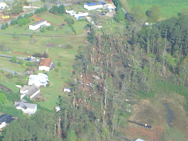
Aerial view of the tornado damage near Double Springs and Townville, South Carolina, on 10 April 2009. Image courtesy of Anderson County Emergency Management.

Author's Note: The following report has not been subjected to the scientific peer review process.

1. Introduction

A series of supercell thunderstorms moved across the upper Savannah River Valley during the afternoon of 10 April 2009, spawning as many as four tornadoes across extreme northeast Georgia and the western portions of Upstate South Carolina. The first tornado touched down at 130 pm Eastern Daylight Time (or 1730 Universal Time Coordinated [UTC]) about one mile west of Long Creek, South Carolina, just over the Georgia state line in western Oconee County. [Note: All times in this document are referenced to UTC. To convert to Eastern Daylight Time, subtract four hours from the UTC time.) The tornado path was only one-tenth of a mile long and damage was rated at EF0 on the Enhanced Fujita Scale. Shortly thereafter, a more powerful tornado tracked across northern Franklin County, Georgia, beginning at 1753 UTC about one mile west of the Red Hill community. This tornado produced damage rated up to EF2 as it moved about 9.5 miles and lifted two miles north northwest of Lavonia at 1806 UTC. The supercell responsible for the Franklin County tornado continued east and produced another tornado over western Anderson County, South Carolina, about six miles south of Townville, beginning at 1823 UTC. The tornado moved across the Lake Hartwell area on a path nearly three miles long and caused damage rated at EF1 intensity before lifting at 1827 UTC. Another weaker tornado touched down in eastern Anderson County at 1853 UTC near Highway 29 and the Jockey Lot.

As the supercells moved into central portions of the Upstate, an evolution to a linear mesoscale convective system (MCS)/bow echo regime was observed in the early part of the evening. This resulted in a perceived transition in the severe weather threat from tornadoes and hail to damaging downburst winds. However, at least five more tornadoes developed in association with bow echoes. Two of them tracked across Abbeville County, South Carolina: one in a rural area three miles northwest of the Watts community (an EF1), and the other across the city of Abbeville (an EF2). At the same time, another tornado (EF1) was on the ground near Jonesville, South Carolina. The final two tornadoes occurred a short while later on the north and south side of Greenwood, South Carolina. Another intermittent path of wind damage also occurred to the south of Monroe, North Carolina, but was determined to be non-tornadic.

Figure 1. Storm Prediction Center (SPC) storm reports for 10 April 2009. Tornado reports are in red. Large hail reports are in green. Damaging straight-line wind reports are in blue. Black squares represent reports of wind gusts of 65 knots or greater. Black triangles are reports of hail 2 inches in diameter or larger.

The forecasters at the National Weather Service (NWS) Forecast Office in Greer, South Carolina, anticipated an outbreak of severe thunderstorms on 10 April 2009. The potential for supercells and tornadoes was also recognized by the Storm Prediction Center (SPC) in the Day 1 Convective Outlook issued at 0559 UTC, which placed northeast Georgia and the western Carolinas in a moderate risk. In fact, the SPC even issued a Public Severe Weather Outlook for the region to highlight the increased danger for significant tornadoes.

2. Synoptic Characteristics

A closed upper low was located over southern Missouri at 500 mb at 1200 UTC on 10 April (Fig. 2). An associated negatively tilted trough axis extended from the low through eastern Arkansas into Mississippi. This resulted in moderately strong and diffluent flow across much of the Tennessee Valley and southern Appalachians. The 300 hPa analysis at 1200 UTC (Fig. 3) revealed the upper tropospheric reflection of the Mississippi Valley low, with a jet maximum moving through the trough axis. Rather strong upper level divergence occurred across the Tennessee Valley in association with the left exit region of this jet streak, although it is possible the divergence may have been augmented by the right entrance region of a second jet maximum across the northeast United States. The analysis also revealed the vertical depth of the diffluent flow pattern over the Tennessee Valley/Southern Appalachian area.

Figure 2. SPC objective analysis of 500 mb geopotential height, temperature and wind at 1200 UTC on 10 April. Click on image to enlarge.

Figure 3. SPC objective analysis of 300 mb isotachs, streamlines, wind barbs, and divergence at 1200 UTC on 10 April. Click on image to enlarge.

The upper air sounding from Peachtree City, Georgia (FFC), at 1200 UTC on 10 April revealed a relatively cool and moist boundary layer (Fig. 4). Despite the early hour, the near-surface environment was relatively well-mixed, due to low-level cloud cover and light southeast surface flow. A shallow temperature inversion was observed between 875 mb and 830 mb. Above this inversion, a shallow layer of very steep lapse rates extended to near the 750 mb level. This layer played a key role in the evolution of convection later in the afternoon across north Georgia and Upstate South Carolina.

Figure 4. Skew-T, log P diagram and wind profile for observed sounding from FFC at 1200 UTC on 10 April. The temperature sounding is shown by the red line and the dewpoint sounding is shown by the dashed green line. A hodograph is provided in the upper left corner. Click on image to enlarge.

Lapse rates diminished in magnitude above the shallow, elevated mixed layer. Surface-based air parcels possessed no potential instability at 1200 UTC due to the cool boundary layer and modest mid-level lapse rates, but wind profiles were quite strong. The flow veered and increased from the surface through 940 mb, with weak veering and strengthening of the flow observed through the remainder of the troposphere. The sounding yielded shear of 23 m s-1 in the 0-3 km layer and 28 m s-1 in the 0-6 km layer, values that were more than adequate for organized storms, including supercells. Storm relative helicity (SRH) values were supportive of rotating updrafts, with SRH exceeding 250 m2 s-2 in the 0-1 km and 0-3 km layers.

The temperature structure in the 875 mb to 750 mb layer in the FFC sounding was a remnant of the elevated mixed layer originating from the high plateau of northern Mexico. The air parcel trajectory analysis in Fig. 5 confirmed the origin of this layer. The role of the elevated mixed layer in severe weather outbreaks across the Great Plains and Mississippi Valley is well-established. However, it has also been discussed in previous analyses of severe weather outbreaks across the western Carolinas and northeast Georgia (Lane, 2008).

Figure 5. Air parcel trajectory analysis from the National Oceanic and Atmospheric Administration (NOAA) Air Resources Lab (ARL) HYSPLIT model. For this analysis, the GDAS model was run backwards for 96 hours from 10 April 2009 at 1200 UTC. Traces show the origin of air parcels at FFC at the 1000 m (red), 2000 m (blue), and 3000 m (green) levels.

At the surface, north Georgia and the Carolinas were located within the warm sector of the low pressure system located over southeast Missouri at 1200 UTC (Fig. 6). A regional surface plot at this time (Fig. 7) indicated air temperatures in the 50s (degrees F) across much of the southeast, while dewpoint temperatures ranged from the 40s across the western Carolinas to the lower 60s near the coasts.

Figure 6. HPC surface fronts and pressure analysis at 1200 UTC on 10 April. Click on image to enlarge.

Figure 7. Surface observations at 1200 UTC on 10 April. Observations are plotted using the traditional station model. Click on image to enlarge.

Another regional plot at 1700 UTC (Fig. 8) revealed how diurnal heating and strong southerly flow affected the low level environment through the morning and early afternoon hours. Air temperatures warmed to the 70s while mixing resulted in an increase in southerly surface winds to 10 to 20 kt across much of the region. However, a small area of the western Carolinas and northeast Georgia had light and variable winds and air temperatures in the upper 50s and lower 60s. This was attributed to weak cold air damming (CAD) that developed in response to stratiform rain falling into the relatively cool and dry airmass that was in place across this area during the morning. Although the main synoptic-scale frontal boundaries remained well west and north of the region, the CAD established a mesoscale differential heating boundary that extended from the central Piedmont of North Carolina, across northern South Carolina, into north Georgia. Fairly strong low-level speed convergence can be inferred along this boundary across the Upper Savannah River Valley.

Figure 8. Surface observations plot at 1700 UTC on 10 April. Click on image to enlarge.

A special upper air observation from FFC taken at 1800 UTC revealed that the structure of the lower atmosphere changed significantly since 1200 UTC (Fig. 9). The combination of heating and large scale upward vertical motion (UVM) beneath the diffluent/divergent upper tropospheric flow resulted in lifting and removal of the low-level inversion seen in Fig. 4. Meanwhile, mid-tropospheric cold advection associated with the upper low and dynamic cooling from UVM resulted in a layer of steep lapse rates between the 720 mb and 600 mb layer. This combination of low-level warm and moist advection, diurnal heating, and steep mid-level lapse rates produced convective available potential energy (CAPE) values in excess of 1300 J kg-1. This was similar to levels of instability associated with previous outbreaks of tornadic supercells across north Georgia and the western Carolinas (Lane, 2008).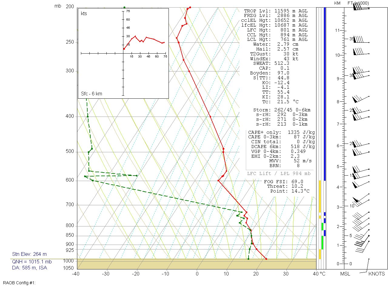

Figure 9. As in Fig. 4, except at 1800 UTC. Click on image to enlarge.

Although mid-tropospheric wind fields strengthened considerably since 1200 UTC, the magnitude of the 0-3 km shear actually diminished to 18 m s-1 due to veering of the surface wind. Meanwhile, the strengthening flow resulted in intensification of the 0-6 km shear to 37 m s-1. Values of SRH remained more than adequate for rotating updrafts, exceeding 200 m2s-2 in both the 0-1 km and 0-3 km layers. Clearly, the combination of instability and shear parameters was supportive of supercells. The potential for isolated tornadoes also existed, particularly from updrafts interacting with the differential heating boundary.

3. Mesoscale Convective Evolution

A band of convection moved from the Tennessee Valley into extreme western North Carolina around daybreak on 10 April. At 1200 UTC, the leading edge of the convective band stretched from metro Atlanta, northward across the western tip of North Carolina, to Morristown, Tennessee (Fig. 10). The line of storms had a history of producing damaging wind gusts and hail as it moved through north Alabama and south central Tennessee but was moving into a less favorable air mass, so additional severe weather potential was thought to be isolated. Although some of the embedded thunderstorms were strong, no severe weather was reported with the convection as it moved across east Tennessee and western North Carolina. The band weakened throughout the morning as it moved across the stable air mass in place across the western Carolinas.

Click here to view a 9 frame loop of a composite reflectivity mosaic from 0900 UTC to 1700 UTC on 10 April.

Figure 10. Regional composite radar reflectivity mosaic at 1200 UTC on 10 April 2009. Click on image to enlarge.

By 1800 UTC, the remnants of the first band of convection extended from the western Piedmont of North Carolina into northern portions of Upstate South Carolina and extreme northeast Georgia (Fig. 11). Although the band of convection had decreased in intensity from 1200 UTC, on the larger scale, isolated strong to severe storms were producing marginally severe hail across northeast Georgia around this time. The SPC mesoscale objective analysis of surface-based CAPE (SBCAPE) at 1800 UTC (Fig. 12) suggested that the convection was elevated, as instability remained non-existent for surface-based air parcels. Meanwhile, another band of convection, with some embedded intense updrafts, was moving across middle Tennessee and extreme northern Alabama in association with the cold front. This convection continued to develop into mostly discrete supercells through the early part of the afternoon, which heightened the severe weather threat for north Georgia. This prompted the issuance of a Tornado Watch (#134) at 1940 UTC for a large area that included far western North Carolina and northeast Georgia. The situation was thought to be particularly dangerous with the potential for long track tornadoes.

Figure 11. Regional composite radar reflectivity mosaic at 1758 UTC on 10 April 2009. Click on image to enlarge.

Figure 12. SPC mesoscale objective analysis of surface-based CAPE (solid brown contours), surface-based convective inhibition (SBCIN, color fill), and surface wind (barbs) at 1800 UTC on 10 April 2009. Click on image to enlarge.

Throughout the afternoon, the differential heating boundary lifted gradually north, as shown by an analysis of SBCAPE at 2200 UTC (Fig. 13). Marginally unstable air, with CAPE values exceeding 500 J kg-1, was moving into extreme northeast Georgia and the lower Piedmont of South Carolina at this time.

Figure 13. As in Fig. 12, except for 2200 UTC. Click on image to enlarge.

As the northern portion of the convective band moved into the more stable air mass across western North Carolina, significant weakening of convection was observed (Fig. 14). However, the southern part of the band remained vigorous, with a well-defined mesoscale convective system (MCS) with bowing reflectivity structures (hereafter referred to as BOW1) moving across north Georgia. Meanwhile, isolated discrete cells were forming along the leading edge of the convective band across extreme northeast Georgia. The environment ahead of the supercells was expected to become increasingly favorable for their maintenance through the early part of the evening. Thus, another Tornado Watch (#135) was issued for Upstate South Carolina at 2231 UTC.

Figure 14. As in Fig. 10, except for 2159 UTC on 10 April 2009. The locations of bow echo 1, supercell 1, and supercell 2 are indicated. Click on image to enlarge.

4. Storm Scale Convective Evolution

Around 2230 UTC, two intense, discrete convective cells were seen on the NWS Doppler radar at the Greenville - Spartanburg International Airport (the KGSP radar). One of the thunderstorms was located over northern Banks County, Georgia, and the other straddled the border between Rabun County, Georgia, and Oconee County, South Carolina (Fig. 15). Both cells exhibited supercellular characteristics, with hook echoes, forward flank inflow notches, moderate to strong mesocyclones, and weak echo regions.

Figure 15. KGSP composite reflectivity at 2229 UTC on 10 April. The color table on the right shows the reflectivity values. Supercells SC1 and SC2 are labelled. Click on image to enlarge.

Despite its impressive structure, large hail up to 4 cm in diameter was the only severe weather reported with the northern supercell (SC1). Examination of Fig. 13, in conjunction with a regional surface plot from 2200 UTC (Fig. 16) provided clues to the absence of tornadoes and damaging winds in association with SC1. These images revealed that SC1 was located 50-60 km north of the differential heating boundary, far into the cool air mass associated with weak CAD. In fact, air temperatures in this area remained in the upper 50s (degrees F). This suggested there was no SBCAPE available to convective updrafts (as confirmed by the SBCAPE analysis in Fig. 13) indicating that the mesocyclonic circulation and any negatively buoyant air were likely to remain aloft.

Figure 16. Regional surface analysis at 2200 UTC on 10 April. The red line denotes the differential heating boundary associated with weak cold air damming.

a. The Franklin County Tornado

Of greater concern was the southern supercell (SC2) in Fig. 15, as this cell was located very close to the surface boundary. As seen in Fig. 13, marginal to moderate values of SBCAPE were slowly spreading northward along the boundary. The KGSP volume scan at 2249 UTC revealed the low-level hook echo and the location of the weak echo region along the border between Stephens County and Franklin County, Georgia (Fig. 17).

The Storm Relative Velocity (SRV) images from this time (Fig. 18) showed the deep, persistent mesocyclone associated with SC2. Rotational velocity (Vr) of 35 kt or greater extended from about 10,000 ft through the 20,000 ft level of this storm. This was well within the moderate mesocyclone category of the mesocyclone detection nomogram. Although the rotation weakened in the lowest elevation scans, there was a broad shear axis at the 0.5 degree scan. Severe weather occurrence was limited to large hail in excess of 4 cm at this point.

Figure 17. KGSP base reflectivity on the (A) 0.5 degree, (B) 1.5 degree, (C) 2.4 degree, and (D) 3.1 degree elevation scans at 2249 UTC on 10 April. The color table is shown in the upper left corner. Click on image to enlarge.

Figure 18. KGSP storm relative velocity on the (A) 0.5 degree, (B) 1.5 degree, (C) 2.4 degree, and (D) 3.1 degree elevation scans at 2249 UTC on 10 April. The color table is shown in the upper left corner. Click on image to enlarge.

Imagery from KGSP at 2258 UTC (Fig. 19) revealed the presence of a rapidly intensifying vortex beneath the mid-level mesoscyclone. Maximum inbound velocity near the hook echo was 90 kt, while the maximum outbound velocity was 50 kt. However, the maxima were not gate-to-gate. Nevertheless, a gate-to-gate shear of 90 kt was present and displaced just to the southwest of the maximum inbound velocity. Rotational shear associated with this velocity couplet was 64.5 x 10-3 s-1, which is off the chart of the rotational shear nomogram, indicating a tornado was probable. At the time of this image, an EF2 tornado was in progress across northern Franklin County (Fig. 20).

Figure 19. KGSP scan at 0.5 degree elevation of (A) base reflectivity, (B) storm relative velocity, and 1.3 degree elevation of (C) base reflectivity and (D) storm relative velocity at 2258 UTC on 10 April. The color table is shown in the upper left corner. Click on image to enlarge.

Figure 20. Track of the Franklin County, Georgia, tornado of 10 April 2009, shown by the solid black line. The tornado began at 2253 UTC and lifted at 2306 UTC. The map scale is shown in the lower left. Click on image to enlarge.

A storm damage survey indicated the tornado lifted before SC2 crossed the South Carolina border.

b. The Anderson County Tornado

Another tornado developed over western Anderson County, South Carolina, after 2300 UTC. A series of images from KGSP at 2327 UTC showed many supercell characteristics during the time of tornado occurrence over Anderson County (Fig. 21). The hook echo remained evident in reflectivity imagery. There was also a rather strong, broad convergent rotational signature at the 0.5 degree elevation scan, indicating the mesocyclone now extended to the lowest levels of SC2. Outbound velocities on the north side of this vortex were very strong, with a maximum of 61 kt. Inbound velocity peaked at 28 kt (Vr of 44 kt, indicating a strong mesocyclone). Embedded within the broader mesocyclonic vortex was a moderately strong gate-to-gate shear of 68 kt. The rotational shear associated with this couplet was 45.4 x 10-3 s-1. Although not as strong as the Franklin County signature, this value also indicated a probable tornado. A short-track, strong EF1 tornado moved across extreme western Anderson County during this time (Fig. 22).

Figure 21. As in Fig. 19, except for 2327 UTC. Click on image to enlarge.

Figure 22. Track of the Anderson County, South Carolina, tornado of 10 April 2009, shown by the solid black line. The tornado began at 2323 UTC and lifted at 2327 UTC. The map scale is shown in the lower left. Click on image to enlarge.

As SC2 moved across Anderson County, SC1 made a transition in convective mode across Pickens County. The environment more favorable for supercells was shifting farther to the south after 2300 UTC. At 2306 UTC, supercell characteristics continued to be observed with SC1, as a hook echo was still seen in the reflectivity field (Fig. 23). The SRV indicated weak, convergent cyclonic shear in association with the hook. However, after 2306 UTC, the rear flank gust front began to surge ahead of the hook, cutting off the inflow into the right flank of the storm. The result of this evolution was seen in the images from KGSP at 2340 UTC (Fig. 24). The reflectivity structure became more elongated. Meanwhile, the SRV indicated the velocity structure of this cell was no longer dominated by cyclonic shear, but rather by a purely convergent signature along the leading edge of the cell, with divergence indicated just upshear of the convergence. In other words, the cell transitioned to an outflow- dominant bow echo as it crossed into Greenville County. At 2345 UTC, a significant downburst event was underway across the west side of the city of Greenville, knocking down dozens of trees. It was somewhat surprising that a strong downburst was able to translate to the surface this far north of the differential heating boundary, especially considering the fact that wind damage was very sporadic as the fully-mature bow echo moved across the remainder of Greenville County, then into Spartanburg County. Surface observations continued to indicate air temperatures in the 50s (degrees F) across northern portions of Upstate South Carolina between 2300 UTC and 0000 UTC while SPC mesoanalysis indicated no SBCAPE that far north. It is speculated that a local weakness in the low-level temperature inversion was present, and that negatively buoyant air possessed sufficient momentum to penetrate this inversion and impact the surface.

Figure 23. KGSP scan at 0.5 degree elevation of (A) base reflectivity, and (B) storm relative velocity at 2306 UTC on 10 April. The color table is shown in the upper left corner. Click on image to enlarge.

Figure 24. As in Fig. 23, except for 2340 UTC on 10 April. Click on image to enlarge.

c. The Jonesville Tornado

From 2355 UTC on 10 April to 0020 UTC on 11 April, the well-developed bow echo moved east across the southern half of Spartanburg County. As the bow echo was poised to move out of Spartanburg County and into Union County, South Carolina, a large area of outbound radial velocity with some values greater than 50 kt at approximately 1000 feet AGL was noted on the 0.5 degree scan from the KGSP radar (Fig. 25). Based upon the radar presentation and a history of wind damage, a Severe Thunderstorm Warning was issued for Union County at 0023 UTC on 11 April.

Figure 25. KGSP base velocity on the 0.5 degree scan at 0022 UTC on 11 April. The warmer colors represent motion away from the radar and the cooler colors show motion toward the radar, as given by the color table on the right. Click on image to enlarge.

The KGSP radar identified a mesocyclone on the 0022 UTC volume scan on the leading edge of the bow echo, although it was difficult to discern a coherent rotational couplet at that time. The 0026 UTC volume scan also contained little information to suggest a tornado was forming, other than broad, cyclonically-convergent rotation on the 1.3 degree to 3.1 degree scans (Fig. 26) on the northern flank of the advancing bow echo. Values for rotational velocity (Fig. 27) and rotational shear (Fig. 28) were similar to previous volume scans with no significant trends noted.

Figure 26. KGSP storm relative motion on the (a) 0.5 degree, (b) 1.3 degree, (c) 2.4 degree, and (d) 3.1 degree elevation scans from the 0026 UTC volume scan on 11 April. Warmer colors represent motion away from the radar and the cooler colors show motion toward the radar, as given by the color table in the middle. Click on image to enlarge.

Figure 27. Rotational velocity on the lowest six elevation scans from the KGSP radar for the period 0022 UTC to 0043 UTC on 11 April. The pink colored region represents the time the tornado was on the ground. Click on image to enlarge.

Figure 28. As in Fig. 27, except for rotational shear. Click on image to enlarge.

With the benefit of hindsight, one can usually identify subtle radar signatures prior to an event that might be considered precursors, and this case is no different. A northward moving boundary can be inferred at 0026 UTC from a line of slightly higher reflectivity on the 0.5 degree scan (Fig. 29) extending from southeast to northwest across Union County and intersecting the convective line over extreme eastern Spartanburg County. This might have allowed slightly more unstable air to advect ahead of the advancing bow echo over Union County. A reflectivity cross-section along the direction of storm motion showed a large echo overhang (Fig. 30), which was even more apparent when viewing a 48 dBZ reflectivity surface generated from the 0026 UTC volume scan (Fig. 31). Although some of the forward tilt might be an artifact of the rapid eastward movement of the storm, the echo overhang suggested a forward-tilting updraft and a weak echo region.

Figure 29. KGSP base reflectivity from the 0.5 degree elevation scan at 0026 UTC on 11 April. The leading edge of the bow echo is indicated as a cold front and the northward moving boundary is indicated as a warm front. The white line shows the location of the reflectivity cross section in Fig. 30. Click on image to enlarge.

Figure 30. Vertical cross section of reflectivity from the KGSP radar at 0026 UTC on 11 April. The location of the cross section is shown by the white line in Fig. 29. Click on image to enlarge.

Figure 31. KGSP radar 48 dBZ reflectivity surface at 0026 UTC on 11 April. The view is to the north normal to the direction of storm motion. Click on image to enlarge.

Although increases in rotational velocity and shear can be considered only modest at best in the scans leading up to tornadogenesis, between 0022 UTC and 0026 UTC a subtle transition from cyclonic convergence toward something closer to pure rotation can be inferred from the storm relative motion on the 2.4 degree and 3.1 degree scans (Fig. 32). On those scans, the radar beam cut through the bow echo between 6500 feet and 8200 feet. The developing rotation at that level was displaced down-shear from the strong convergence observed on the 0.5 degree scan, shown by the black "X" on Fig. 26.

Figure 32. KGSP storm relative motion on the 2.4 degree elevation scan at (a) 0022 UTC and (b) 0026 UTC, and on the 3.1 degree elevation scan at (c) 0022 UTC and (d) 0026 UTC on 11 April. The color scale is given in the center of the figure. Click on image to enlarge.

A rapidly-tightening rotational couplet was observed on the 1.3 degree and 2.4 degree scans at 0031 UTC (Fig. 33). Although no significant increase in maximum rotational velocity (Fig. 27) was seen on any scan up to 0031 UTC, the rotational shear (Fig. 28) increased dramatically on the 1.3 degree and 1.8 degree scans at that time. The rotational shear more than doubled on the 1.3 degree scan to a value of 0.047 s-1, which was well within the "tornado likely" region of the rotational shear nomogram for a storm located 25 nm from the radar. This information arrived too late to effectively upgrade Union County to a Tornado Warning as the tornado touched down at 0032 UTC.

Figure 33. As in Fig. 26, except for 0031 UTC on 11 April. Click on image to enlarge.

The tornado was already on the ground at 0035 UTC (Fig. 34) when the KGSP radar clearly indicated the presence of the tornado to the south of Jonesville (Fig. 35). A gate-to-gate couplet with a rotational velocity of 54 kt was seen on the two lowest elevation cuts. Rotational shear was well off the chart.

Figure 34. Approximate track of the Jonesville tornado from 0032 UTC to 0038 UTC on 11 April. The tornado first touched down near Zig Zag Road and Proctor Road and lifted near the MIlliken plant on Bob Little Road. Click on image to enlarge.

Figure 35. KGSP storm relative motion on the 0.5 degree elevation scan at 0035 UTC on 11 April. Click on image to enlarge.

The bow echo surged forward at low levels over west-central Union County between 0026 UTC and 0035 UTC, which could be seen in the base velocity as a bulge in outbound radial velocity (Fig. 36). The forward surge deformed the bow echo to the north of its apex with a rotational couplet (which was in fact a mesovortex) located at an inflection point on the bow (Fig. 37). That the bow echo had the appearance of the familiar "S-shape" seen in cool season high shear, low instability environments may be more than mere coincidence. The surge was probably caused by a rear inflow jet, manifested by the channel of lower reflectivity wrapping in from behind the bow echo which appeared in 44 dBZ reflectivity surfaces (not shown). The rear inflow jet dessicated the higher reflectivity at low levels between 0026 UTC and 0039 UTC which suggested descent. The weak echo channel wrapped around the position of the rotation seen at 6000 to 8000 feet AGL minutes before the tornado touched down. The descending rear inflow jet may have induced cyclonic vorticity at low levels to the north of its core and underneath the rotation seen on the 2.4 degree and 3.1 degree scans. This would provide a means for extending a tornadic vortex down to the surface.

Figure 36. KGSP base velocity on the 0.5 degree elevation scan at (a) 0026 UTC, (b) 0031 UTC, (c) 0035 UTC, and (d) 0039 UTC on 11 April. Red shades represent motion away from the radar and green shades show motion toward the radar. Click on image to enlarge.

Figure 37. Position of leading edge of bow echo observed in 0.5 degree radial velocity in KGSP radar data from 0026 UTC to 0039 UTC on 11 April. The location of the mesovortex is shown by the green line.

As quickly as the rotation appeared on KGSP, it diminished by 0039 UTC as the tornado had already lifted. No further damage was reported in Union County, although the storm continued to produce wind damage across parts of York County and Chester County.

d. The Abbeville Tornado

Meanwhile, a bow echo (BOW1 in Fig. 14) continued to intensify as it moved across north Georgia and the lower piedmont of South Carolina during the early evening. Because this area was south of the differential heating boundary, at least marginal SBCAPE was present, and there was no question about negatively buoyant air reaching the surface. Indeed, downburst damage was fairly widespread as this bow echo moved across Elbert County, Georgia, and western portions of Abbeville County, South Carolina. A brief tornado was spawned over western Abbeville County along Old Calhoun Falls Road near the community of Watts between 0023 UTC and 0025 UTC.

The well-organized MCS/bow echo was located over central Abbeville County at 0026 UTC on 11 April (Fig. 38). The SRV revealed an elongated axis of cyclonic shear along the leading edge of the higher reflectivity. However, this shear evolved into a broad area of rotation associated with a forward flank inflow notch just north of the bowing segment. Vertical analysis of the velocity structure indicated this was not a mesocyclone, since the rotation weakened with height, but was more likely the bookend vortex associated with a mature bow echo. With time, this circulation would intensify. In fact, at 0035 UTC a gate-to-gate shear couplet of 74 kt was evident just north of the apex of the bowing segment (Fig. 39). The rotational shear associated with this vortex was 55.2 x10-3 s-1, well within the "tornado probable" category of the rotational shear nomogram. Around the time of this image, an EF2 tornado caused extensive damage across the city of Abbeville (Fig. 40).

Figure 38. As in Fig. 23, except for 0026 UTC on 11 April. Click on image to enlarge.

Figure 39. As in Fig. 23, except for 0035 UTC on 11 April. Click on image to enlarge.

Figure 40. Track of the Abbeville, South Carolina, tornado of 10 April 2009, shown by the solid black line. The tornado touched down at 0028 UTC and lifted at 0036 UTC on 11 April. The map scale is shown in the lower left. Click on image to enlarge.

Despite the non-supercell nature of the Abbeville storm, a successful Tornado Warning (TOR), with about 15 minutes of lead time was issued for this event, based partly upon the rotation associated with the bookend vortex, but also upon environmental considerations. This storm was clearly located on the warm side of the differential heating boundary, and was therefore surface-based. Concerns about the potential of the parent updraft to tilt and stretch baroclinically generated horizontal vorticity in the vicinity of the surface boundary prompted TOR issuance.

e. The Greenwood Tornadoes

The bow echo that produced the Abbeville tornado continued to move quickly east and into Greenwood County, South Carolina, after 0045 UTC. The final two tornadoes of the event spun up on the leading edge of the QLCS as it moved across the city of Greenwood around 0048 UTC (Fig. 41). The first tornado touched down west of Greenwood and traveled east- southeast across the southern part of the city (Fig. 42). The second tornado touched down on the northeast side of the city, just two minutes after the first, and moved east.

Figure 41. KGSP base reflectivity (top) and storm relative motion (bottom) on the 0.5 degree scan at 0048 UTC on 11 April. Click on images to enlarge.

Figure 42. Track of the Greenwood, South Carolina, tornadoes of 10 April 2009, shown by the solid black lines. The southern tornado touched down first at 0041 UTC and lifted at 0047 UTC on 11 April. The northern tornado touched down second at 0043 UTC and ended at 0045 UTC. The map scale is shown in the lower left. Click on image to enlarge.

f. The Union County, North Carolina, Storm

By 0100 UTC, the transition to a linear convective system was nearly complete, suggesting the primary threat for the area downstream was damaging winds.

The bow echo remnant of the storm that produced the tornado near Jonesville moved south of Charlotte around 0130 UTC. The KGSP radar showed the leading edge of the bow echo entering Union County, North Carolina, at 0135 UTC (Fig. 43). The bow echo appeared to weaken through 0148 UTC over the southwestern part of the county. By 0151 UTC, the bow echo moved far enough away from the radar that storm relative motion data was not available. Radar data from the Terminal Doppler Weather Radar located north of the Charlotte - Douglas International Airport (the TCLT radar) was contaminated by improperly dealiased velocity information and yielded few clues about the potential for additional severe weather. Meanwhile, the NWS Doppler radar at the Columbia, South Carolina, airport (the KCAE radar) was close enough to have a good view of the bow echo as it moved south of Charlotte. The KCAE radar showed evidence of the bow echo remnant to the south of Monroe, North Carolina, but did not detect any coherent rotational signature on the 0.5 degree scan (Fig. 44).

Figure 43. KGSP radar reflectivity at (A) 0.5 degrees, (B) 0.9 degrees, (C) 1.3 degrees, and (D) 1.8 degrees from the 0130 UTC volume scan on 11 April. Click on image to enlarge.

Figure 44. KCAE base reflectivity (top) and storm relative motion (bottom) on the 0.5 degree scan at 0149 UTC on 11 April. Click on images to enlarge.

The weakened bow echo produced a straight but intermittent path of tree, outbuilding, and roof shingle damage about five miles south of Monroe. The damage path was on the order of two miles long and about one-quarter mile wide. However, the majority of the trees were blown down in the same general direction. Damage to structures was on the windward side with any debris blown in the direction of storm travel. A group of 10 Bradford pear trees lining a driveway were all blown down in the same direction and a metal carport behind a house was lifted up and blown onto the back deck of the house. There was some evidence here to suggest the trees were on the south side of the damage path and blown in a direction that would be convergent with the storm track.

The preponderance of radar evidence from KGSP, KCAE, and TCLT suggested a bow echo and collapsing updraft/elevated reflectivity core near the spot where the damage began. For that reason, the subjective interpretation of the damage was that it was caused by straight-line wind and not a tornado.

5. Concluding Remarks

The tornado outbreak on 10 April 2009 was a challenging event, particularly because the nature of the convection transitioned from supercellular during the late afternoon, to quasi-linear convective systems (QLCS) during the evening. The Jonesville and Abbeville tornadoes were essentially QLCS tornadoes spawned from a low level mesovortex (see Weisman and Trapp 2003 for an overview of mesovortices). Atkins and St. Laurent (2009) found that stronger and potentially more damaging mesovortices occurred when low level shear was nearly balanced by horizontal vorticity generated by the cold pool, which also resulted in upright updrafts. The scientific literature has many examples of tornadoes along the edge of bow echoes. Some studies (especially DeWald and Funk 2000 ) have noted tornadogenesis associated with rapid spin-up of well-defined cyclonic circulations from transient low-level shear zones along and to the north of the apex of a bowing convective line segment. Other authors note the difficulty that similar rapid intensification and tornadogenesis imposes on the issuance of effective warnings.

References

Atkins, N. T., and M. St. Laurent, 2009:  Bow echo mesovortices.  Part 1:  
     Processes that influence their damaging potential.  Manuscript 
     submitted to Monthly Weather Review for publication.


DeWald, V. L., and T. W. Funk, 2000: WSR-88D reflectivity and velocity 
     trends of a damaging squall line event on 20 April 1996 over south-
     central Indiana and central Kentucky. Preprints, 20th Conf. on 
     Severe Local Storms, Orlando, FL, Amer. Meteor. Soc., 177-180.

Weisman, M. L., and R. J. Trapp, 2003:  Low-level mesovortices within 
     squall lines and bow echoes.  Part 1:  Overview and dependence on 
     environmental shear.  Mon. Wea. Rev., 131, 2779-2803.

Acknowledgements

The KGSP radar images were created using the Java NEXRAD viewer obtained from the National Climatic Data Center. Other KGSP radar views, including reflectivity cross sections and reflectivity surfaces were created using the GRlevel2 Analyst software package. Satellite imagery, radar mosaics, and surface observation plots were obtained from the RAP Real-Time Weather page maintained by the University Corporation for Atmospheric Research. Upper air analyses and mesoscale analyses were obtained from the Storm Prediction Center. Upper air sounding plots were created using the RAwinsonde OBservation (RAOB) Program (version 5.8) for Windows. The surface analyses were obtained from the Hydrometeorological Prediction Center. Tornado track images were created using DeLorme Street Atlas USA 2009 edition.