
A late season winter storm will produce a combination of heavy snow and disruptive ice starting this evening in the Northern Plains and moving into the Upper Midwest and Great Lakes by tonight continuing through Thursday. Severe thunderstorms will likely produce severe wind gusts, large hail, a few tornadoes, and heavy rainfall across the southern and central Plains today. Read More >
A Look Back at the Western Carolina Violent Tornado Outbreak
of 5 May 1989
|
|
|
Fig 1. Reports of severe weather on 5 May 1989. See map legend for key. Click here to launch interactive map in new tab. |
I. Introduction
One of the worst tornado outbreaks in the history of the western Carolinas occurred on 5 May 1989. While only seven tornadoes were reported across the area during the outbreak, three were rated F4 in intensity (Fig. 1). This number of violent tornadoes is unprecedented for a single outbreak affecting the region since official records began in 1950[1]. By contrast, only a single F4 (or EF4) tornado has affected the area since this time[2]. The 5 May 1989 tornadoes produced around $40 million in damage (adjusted to 2012 dollars), making this the most damaging tornado outbreak in the area since at least 1950. Seven people were killed and over 100 injured, reflecting the most casualties during a single western Carolina tornado outbreak since 16 April 1944. The tornado that moved through portions of northern Cleveland, northwest Lincoln, and southwest Catawba counties in North Carolina was arguably the strongest tornado known to have affected the region, as 4 fatalities, over 50 injuries, and $10 million in damage (adjusted to 2013 dollars) occurred, despite this being a largely rural area. The paucity in violent tornado occurrence observed across the area during the past 25 years may have created a false sense of security, not only among the public, but among forecasters responsible for warning the public of the threat (long term and immediate) of destructive tornadoes. The purpose of this document is three-fold. An historical overview of the nature of National Weather Service (NWS) operations in 1989 will be included in Section 2. Section 3 will contain a scientific discussion of the synoptic and mesoscale environmental characteristics that supported intense tornadoes on 5 May 1989. Section 4 will detail the public impacts of two of the three violent tornadoes, including witness testimony. Lessons learned and a summary and conclusions will be included in Section 5.
2. National Weather Service Operations in 1989
The NWS experienced a major restructuring in the mid-1990s that saw the number of Weather Service Forecast Offices (WSFOs) increase two-fold, while hundreds of “satellite offices,” dubbed Weather Service Offices (WSOs) were all but eliminated. Prior to the modernization, the WSOs were tasked with “short-fuse” warning (i.e., Severe Thunderstorm, Tornado, and Flash Flood) responsibility, typically for around a dozen counties. In 1989, five WSOs and one WSFO shared warning responsibility for the 46 counties comprising the current Greenville-Spartanburg County Warning Area (CWA; Fig. 2). In addition, the Storm Prediction Center (SPC), now in Norman, OK, was located in Kansas City, MO, and was known as the National Severe Storms Forecast Center (NSSFC).

|
Fig. 2. County Warning Areas of NWS Weather Service Offices (WSOs) in the western Carolinas and northeast Georgia in 1989.
|
Technology available to NWS forecasters was dramatically different in 1989. Operational implementation of Next Generation Weather Radar (NEXRAD) with Doppler velocity retrieval capability was several years away. Forecasters were therefore unable to objectively observe storm-scale rotation. Storm severity had to be inferred from the amount of power returned (reflectivity) to the radar by reflectors (i.e., rain and hail) within a storm, while tornadic potential could only be diagnosed via the reflectivity pattern. In addition, the coverage provided by the radar network was much poorer in 1989 (Fig. 3) than today. Less than half of the WSOs were collocated with radars. WSOs that were not collocated with a radar usually had access to a phone line feeding images from the closest “network radar” (WSR-57 and WSR-74S radars in Fig. 3). However, these radars were sometimes located too far from CWAs to provide quality data (Fig. 5). For instance, only three “network” radars were operational in Georgia and the Carolinas, with two of those being along the coast. Network radars providing primary coverage to the Western Carolinas were located in Bristol, TN and Athens, GA. Data availability was often unreliable, especially during periods of severe weather. Manual operation of the radar by NWS personnel at the parent office was a tedious process that often resulted in a 15-20 minute delay in data availability. (Jones, personal communication) This made the data more or less useless for warning decision making purposes during a significant event. Forecasters essentially used this obsolete data to estimate the current location of the storm and to forecast its movement. Meanwhile, warning decisions were based largely upon storm history and on reports of damage, funnel clouds, wall clouds, etc.
 |
 |
||
|
Figure 3. The NWS radar network in 1989. Rings |
Figure 4. Same as in Fig. 3 except for the modern |
As a supplement to the network radars, some WSOs and many WSFOs were collocated with “local” WSR-74C radars. These “C-band” radars operated at 5-cm wavelength and therefore had limited range and were subject to severe data degradation (i.e., attenuation), especially when storms were located near the radar. More importantly, their data were only available to the parent office. This required personnel at the parent office to proactively communicate significant radar features associated with storms in other CWAs to neighboring WSOs. Overall, the warning process was by necessity much more reactive 25 years ago than it is today. The probability that even a large and destructive tornado would be preceded by a Tornado Warning was only around 50%. If a warning was issued, lead time was only a couple of minutes at best for the initial point of touchdown.
 |
 |
||
|
Figure 5. Radar image from the Bristol, TN (TRI)
|
Figure 6. Manual radar observations from TRI |
3. Synoptic and Mesoscale Overview of 5 May 1989
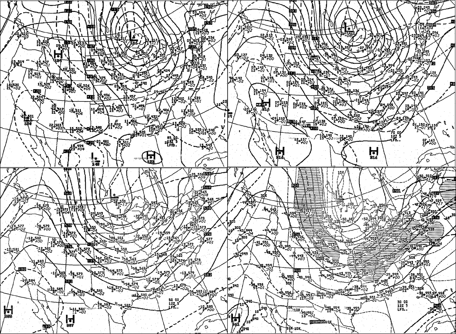
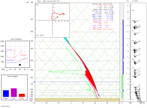
Upper level low pressure was located over the Midwest at 1200 UTC on 5 May 1989 (Fig. 7 (lower left)). A trough with a slight negative tilt extended from the upper low down the Mississippi Valley. A core of strong upper level winds in excess of 50 m/s was centered over the Ohio Valley. At 1500 UTC[3], a strong area of low pressure was observed at the surface across the northern Great Lakes (Fig. 9). A weaker, smaller area of low pressure (i.e., a meso-low) was centered over central Mississippi. The synoptic pattern generally fit the “Great Lakes” composite pattern sometimes associated with significant tornadoes in the western Carolinas and northeast Georgia (Lane, 2008). The 1200 UTC rawinsonde observation (RAOB) from Jackson, MS (JAN; Fig. 8) was the sounding that was most likely representative of the synoptic scale conditions associated with tornadic convection across the western Carolinas late in the day on 5 May 1989. Weak lapse rates through the depth of the troposphere were resulting in a stable sounding, as even most unstable CAPE (MUCAPE) was 0 J/kg. However, wind profiles were very strong, with strong clockwise turning observed in the lowest 1.0 km AGL. A rapid increase in wind speed was also noted, with the core of a low level jet of 25 m/s observed around the 1.0 km level. As a result, shear magnitude in this layer was 24 m/s, while Storm Relative Helicity (SRH) was 425 m2 s-2. Wind speeds increased further above 3.0 km AGL, with 39 m/s of flow observed at 6.0 km AGL. Zero-to-6 km shear magnitude was 38 m/s. It should be noted that the winds in the JAN sounding were anomalously strong at 1200 UTC, especially for sounding locations downstream of the upper trough axis. Wind speeds diminished significantly in all directions from JAN. This may have been an indication that wind speeds were locally enhanced in the vicinity of the mesolow and an associated mesoscale vorticity center (MVC). The anomalously warm air at 500 hPa at JAN was most likely a reflection of the MCV.
 |
 |
 |
|
Figure 7. Figure 4. Rawinsonde observations and analyses at 850 hPa (upper left), 700 hPa (upper right), 500 hPa (lower left), and 300 hPa (lower right) at 1200 UTC on 5 May 1989. |
Figure 8. Sounding of rawinsonde observation from Jackson, MS at 1200 UTC on 5 May1989. |
Figure 9. Surface observations and analysis from 1500 UTC on 5 May 1989. |
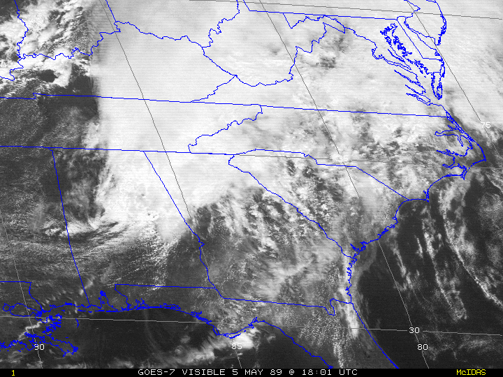
By 1800 UTC on 5 May 1989, the mesolow and associated surface boundary had moved rapidly east/northeast to the Alabama/Georgia border west of the Atlanta area. This mesoscale system had moved well east of the synoptic boundary (Fig. 10). A weak thermal boundary, likely delineating rain-cooled air from the warm sector air mass extended east /northeast from the mesolow across north Georgia, Upstate South Carolina, into central North Carolina. The air mass on the “cool” side of this thermal boundary was modestly unstable according to a sounding from Upstate South Carolina reconstructed from National Centers for Environmental Prediction (NCEP) reanalysis data at 1800 UTC (Fig. 11). Zero-to-one km mixed layer CAPE (MLCAPE) was 660 J/kg, while MLCAPE within the 0-3 km layer was 187 J/kg. The wind profile was not nearly as strong as that observed at JAN at 1200 UTC, perhaps not surprising considering that the mesolow system was still approximately 300 km to the west/southwest. Nevertheless, conditions were becoming favorable for supercells and tornadoes across the western Carolinas owing to adequate CAPE and shear/SRH parameters. In fact, the Significant Tornado Parameter (STP) was above the optimal 1.0 level. Low infrared (IR) satellite temperatures implied large scale forcing for upward vertical velocity (UVV) across much of the Tennessee Valley and southern Appalachians (Fig. 12), although visible imagery did not reveal any areas of intense convection over the region at this time (Fig. 13)
|
|
 |
 |
|
|
Figure 10. Same as in Fig. 9 except at 1800 UTC. |
Figure 11. Sounding constructed from NCEP reanalysis data and modified for surface observations at the Greenville-Spartanburg Airport (GSP) at 1800 UTC on 5 May 1989. The data are from a grid point approximately 29 km WNW of GSP. |
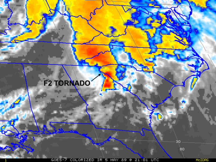
Citing the rapid advancement of the mesolow system into a destabilizing air mass, which was expected to result in a rapid increase in thunderstorm activity, the NSSFC issued Tornado Watch 183 for much of north and central Georgia and the northwest corner of South Carolina at 1821 UTC (Fig. 14), valid until 0100 UTC on 6 May 1989. Indeed, explosive thunderstorm development occurred in the form of a quasi-linear convective system (QLCS) along the surface boundary across north and central Georgia after 2000 UTC (Fig. 17). The first tornado of the event, associated with a cell in the northern portion of the QLCS (Jones, personal communication) and eventually rated F1, was reported near Gainesville, GA at around 2030 UTC. The cell responsible for this tornado subsequently produced an F2 tornado near Toccoa, GA in Stephens County, and two F1 tornadoes in Oconee County, South Carolina: one in the Madison community, and the other near Tamassee. The explosive convective development and reports of these initial tornadoes prompted NSSFC to issue another Tornado Watch (185) at 2033 UTC for much of South Carolina and portions of western and central North Carolina (Fig. 15). The Tornado Watch contained “Particularly Dangerous Situation (PDS)” wording, mentioning “the possibility of very damaging tornadoes.” “PDS” watches are quite rare, especially in the Southeast (Fig. 16).
 |
 |
 |
|
Figure 12. GOES visible satellite imagery from 1801 UTC on 5 May 1989. Click here for a loop of infrared imagery. |
Figure 13. GOES infrared satellite imagery from 1801 UTC on 5 May 1989. Click here for a loop of visible imagery. |
Figure 14. Tornado Watch number 183 issued at 1821 UTC on 5 May 1989. |
 |
 |
 |
|
Figure 15. “PDS” Tornado Watch number 185 issued at 2033 UTC on 5 May 1989. Click here for the watch text. |
Figure 16. United States “PDS” Tornado Watch Frequency 1996-2005. From Dean and Schaefer (2008). |
Figure 17. Same as in Fig. 12 except at 2101 UTC. The approximate location of an F2 tornado near Toccoa, GA is labeled, having occurred shortly before the time of this image. Click here for a loop of infrared imagery. |
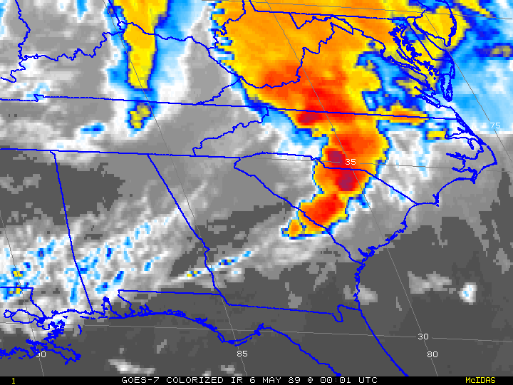
By 0000 UTC on 6 May 1989, the mesolow was located near Greensboro, NC (Fig. 18). It had moved approximately 1000 km in 12 hours, an average speed of approximately 26 m s-1. The 0000 UTC RAOB from Greensboro (KGSO; Fig. 19) revealed intense wind fields in the vicinity of the mesolow. SRH was 475 m2 s-2 in the 0-1 km layer and 601 m2 s-2 from 0-3 km. Zero-to-one kilometer wind shear was 22.6 m s-1. Instability remained marginal across the region, as MLCAPE was only 510 J/kg. Nevertheless, the very strong shear parameters were resulting in composite parameter values very favorable for supercells and significant tornadoes. The STP was 3.7, well above the optimal value of 1.0. This environment continued to support intense convection (Fig. 20), particularly with a tornadic cell near Monroe, NC.
 |
 |
 |
|
Figure 18. Same as in Fig. 9 except at 00Z on 6 May 1989. |
Figure 19. Sounding of rawinsonde observation from Greensboro, NC at 0000 UTC on 6 May1989. |
Figure 20. Same as in Fig. 12 except at 0001 UTC on 6 May 1989. Click here for a loop of infrared imagery.
|
4. The Violent Tornadoes of 5 May 1989
The first violent tornado on 5 May 1989 occurred in association with a discrete supercell thunderstorm that developed ahead of the QLCS over Upstate South Carolina. According to WSO Greer, SC (GSP) personnel, the cell was very small and not especially reflective in radar data. Witnesses also reported little in the way of rainfall beneath the cell, leading to speculation that it was a “low precipitation (LP)” supercell (Jones, personal communication). This would be an extraordinarily rare event for the Carolinas, as these phenomena are usually associated with the dry environs of the central United States’ High Plains. In addition, LP supercells are usually not tornadic, as the storm-scale thermal gradients associated with precipitation are important for tornadogenesis. Nevertheless, a funnel cloud was reported with this cell near Boiling Springs, SC at around 1815 EDT. WSO Greer, SC issued a Tornado Warning based upon this report at 1818 EST. A large tornado (more than 400 yards in diameter, referred to hereafter as the Chesnee Tornado) touched down around 1820 EDT about six miles southwest of Chesnee, between Parris Bridge Road and Peachtree Road, just south of Rainbow Lake. The tornado moved rapidly northeast, initially paralleling Parris Bridge Road. By the time it reached Rainbow Lake, it had expanded to near 1000 yards and was producing at least F2 damage (Fig. 21).
The first fatality of the event occurred near the intersection of Martin Camp Road and Parris Bridge Road (about 3 miles WSW of Chesnee) where a 66-year-old man was killed when his home’s chimney fell on top of him (Fig. 22). The tornado continued to move north/northeast over a largely rural area, passing within two miles west of downtown Chesnee. Several mobile homes were completely destroyed after being tossed hundreds of feet along Turkey Farm Road (Fig. 23). The tornado was most destructive near Highway 11 just northwest of Chesnee (the Arrowood community), where F4 damage was assigned to at least one home (Fig. 24). The intense tornado moved rapidly (estimated 50 to 60 mph) toward extreme northwest Cherokee County, crossing the county line near Old Island Ford Road. A 59-year-old woman was killed in this area, apparently as she was attempting to flee her mobile home which was “disintegrated” by the tornado (Fig. 25). The tornado continued to produce significant damage after crossing into Rutherford County, NC in the vicinity of Montgomery Drive. It continued north/northeast before lifting near Henrietta at around 1835 EDT. Thirty-one mobile homes were damaged or destroyed by the tornado. Twenty-nine houses were destroyed and 78 damaged. This was extensive damage considering the rural nature of the area affected. In addition to the two fatalities, 35 people were injured.
 |
 |
 |
|
| Figure 21. Several cottages were destroyed on Rainbow Lake. Residents of the area could not explain the origin of the bale of hay (lower left), estimated to weigh as much as 1000 pounds. Photo courtesy of Wes Tyler, South Carolina State Climate Office. | Figure 22. F2/F3 damage to a home on Martin Camp Road. A 66-year-old man was killed here when the chimney fell on him. Photo courtesy of Wes Tyler, South Carolina State Climate Office. | Figure 23. Several mobile homes were swept away on Turkey Farm Road. All that was left of this home were the concrete stairs, with rubble thrown more than a 100 feet away. Photo courtesy of Wes Tyler, South Carolina State Climate Office. | Figure 24. Several high tension towers were toppled west of Chesnee. These were designed to withstand wind speeds of at least 100 mph. Photo courtesy of Wes Tyler, South Carolina State Climate Office. |
 |
 |
 |
 |
| Figure 25. Probable F4 damage to a brick veneer home in the Arrowood community. This is a reprint from the Storm Data publication, as the originals could not be found. Original photo by Wes Tyler, South Carolina State Climate Office. | Figure 26. Another mobile home lifted and tossed by the tornado, this one on Old Island Ford Road north of Chesnee. A 59-year-old woman was killed at this location. Photo courtesy of Wes Tyler, South Carolina State Climate Office. | Figure 27. A classic example of wood debris acting as a missile. Exact location of the photo is unknown, but this is probably west of Chesnee. Photo courtesy of Wes Tyler, South Carolina State Climate Office. | Figure 28. Another "wood missile" example. Photo courtesy of Wes Tyler, South Carolina State Climate Office. |
The supercell responsible for the Chesnee tornado moved quickly northeast across eastern Rutherford and west central Cleveland County, but no severe weather was reported. Despite the devastation that had occurred near Chesnee, and an awareness of the severe weather potential, emergency preparedness officials in Cleveland County, NC had little inkling that a storm with a history of producing a violent tornado was bearing down on their county (Cook, personal communication). In fact, by the time a Tornado Warning was issued by WSO Charlotte, another F4 tornado had already ravaged portions of the Lawndale and Vale areas in Cleveland and Lincoln counties. The tornado touched down two to three miles north/northwest of Lawndale (or about 11 miles north/northwest of Shelby), along Mauney Rd. The tornado moved rapidly north/northeast and quickly evolved into a large, multiple vortex tornado as it approached Casar-Lawndale Road.
“[A home in the 800 block of] Casar-Lawndale Rd was the first house to be destroyed[4], and I remember him saying it was a multi-vortex tornado coming toward them. It removed their log home (completely destroyed, Fig. 29) from the foundation with them in the basement. He had a power company line truck that it rolled down through the field about 300 yards from their house.”
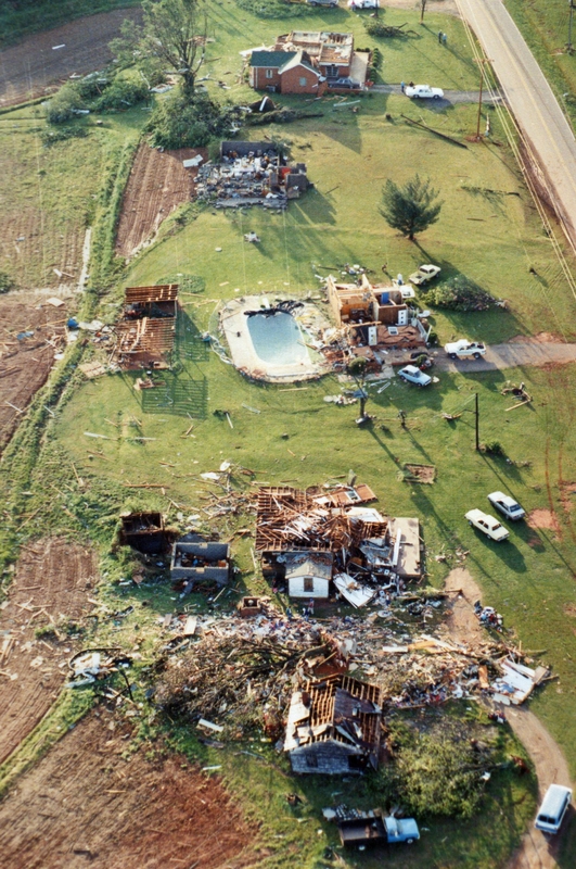
The tornado moved north/northeast at 50 to 60 mph, destroying a home and several outbuildings on Elam Road (Fig. 30). The tornado continued north/northeast over largely rural areas across Warlick Road, Carpenters Grove Church Road, Queen Road, and Sandpit Road, destroying or severely damaging what few buildings stood in its path. One house on Queen Road was removed from its slab foundation and tossed about 100 yards. The tornado reached maximum size (at least a half mile in diameter) and intensity as it moved through the Toluca community on the Lincoln/Cleveland county line, especially near the Highway 18/Highway 27 intersection, where every building within about a quarter mile was heavily damaged or completely destroyed (Figs. 31 and 32). This included several well-constructed frame houses (Fig. 32). Vehicles traveling along Highways 18 were tossed more than 200 yards (Fig. 33), and three of the four fatalities that occurred in this area were in vehicles.
“My co-worker and her husband were traveling on Highway. 18 South when she said it was like hitting a dark wall of water. She was thrown through the sunroof of the car, landing in a field. She saw cows being thrown around but everything around her was gone. She saw red lights in the far distance (Highway 27). Her back was broken. Her husband was killed in the car, where several cars were in a pile in front of Sain's Barber Shop (Highway 18 between Highways 10 and 27).”
Although the tornado began to weaken as it moved across extreme northwest Lincoln County, it continued to produce F2 or F3 damage along Highway 10 (Fig. 34). The tornado continued into southwest Catawba County before lifting in the Propst community. In addition to the 4 fatalities (all in the Toluca community), the tornado was responsible for 52 injuries. A total of 40 houses and 11 mobile homes were destroyed. Fifty-three additional houses and ten mobile homes were damaged. Total monetary damage was estimated at $6 million (adjusted for 2013 dollars). Again, this was extensive damage considering the rural nature of the area.
 |
 |
 |
|
Figure 29. A log home on Casar Lawndale Rd was one of the first to be destroyed by the tornado. Photo courtesy of Gene Meade, Casar, NC/Shelby Civil Air Patrol. |
Figure 30. This home and several adjacent outbuildings were destroyed on Elam Road. Photo courtesy of Gene Meade, Casar, NC/Shelby Civil Air Patrol. |
Figure 31. A church was destroyed along Highway 18 in the Toluca community. Photo courtesy of Gene Meade, Casar, NC and Cleveland County Emergency Management. |
 |
 |
 |
|
Figure 32. F4 damage to a home on Highway 18, just north of Highway 27 on the Cleveland/Lincoln county line. Photo courtesy of Gene Meade, Casar, NC/Shelby Civil Air Patrol. |
Figure 33. Several vehicles were lifted and tossed hundreds of yards. Three of the four fatalities associated with the tornado occurred in vehicles (all in the Toluca community). Photo courtesy of Dwayne Martin, Hickory, NC. |
Figure 34. The tornado appeared to weaken as it left Highway 18, moving along Highway 10 in northwest Lincoln County, but was still producing at least F2 damage. Photo courtesy of Gene Meade, Casar, NC/Shelby Civil Air Patrol. |
5. Conclusion
Advances in technology have revolutionized all aspects of the weather warning system over the past 25 years. The NEXRAD network, implemented in the mid-90s increased radar coverage across the United States, but more importantly introduced Doppler technology, which provided forecasters with information about the radar-relative wind flow within thunderstorms. This enabled forecasters to detect thunderstorm mesocyclones, which were found to sometimes precede tornado development by 30 minutes or more. The process of issuing warnings therefore became much more proactive and slightly more forecast-based than in the pre-modernization era. The result has been vastly improved lead times and detection probabilities of tornadoes (Figs. 35 and 36). This is especially true of strong and violent tornadoes. Since the vast majority of strong tornadoes are preceded by strong mesocyclones, the probability of an EF3 or stronger tornado being preceded with a Tornado Warning is over 90%. Typical Tornado Warning lead time for these strong tornadoes is over 20 minutes, which is about a 300% improvement from 25 years ago. In other words, it would now be extremely rare for the types of violent tornadoes that affected the region on 5 May 1989 to occur with little or no warning.
|
|
 |
 |
|
|
Figure 35. Probability of a tornado (left series) or |
Figure 36. Same as in Fig. 33 except for average lead time.
|
Of equal importance is the improvement in communication technology that has streamlined the warning dissemination process. Activation of the Emergency Alert System is automatic and practically instantaneous once a forecaster issues a warning. Cell phone technology, the internet, social media, and other technological innovations have expanded access to and timeliness of information, including that of storm damage reports. Unlike the long delays in reception of damage information that occurred on 5 May 1989, it would be almost unheard of today for reports of major damage to not “fan out” to downstream interests in a matter of minutes or even seconds. Nevertheless, this event, and similar events in the historical record (Table 1) prove that that there is a need for operational forecasters, as well as those in the public to prepare for the inevitability of these types of tornadoes occurring again. There have been several close calls throughout the years, most recently during the 27 April 2011 historic tornado outbreak. Although several weak tornadoes occurred in the western Carolinas during this event, including a killer EF-3 tornado that ravaged portions of the northeast Georgia Mountains, the area was spared the brunt of this event. However, an objective examination of the data indicates that this was likely only a matter of timing. Since the storm system responsible for the outbreak began to affect the area during the late evening and early morning hours, instability had begun to wane, allowing the severity of the storms to diminish. If the storm system responsible for this event had been only 3 or 4 hours “faster,” the western Carolinas and northeast Georgia may have been at the “epicenter” of this historic outbreak of violent tornadoes.
| County(s) | Rating | Date | Time |
| Union, NC | F3 | 19 Feb 1884 | 2000 |
| Union, NC/Anson, NC/Stanly, NC | F4 | 12 Apr 1920 | 2100 |
| Alexander, NC | F3 | 18 May 1922 | 1845 |
| Pickens, SC | F3 | 13 Mar 1929 | 2030 |
| Anderson, SC/Greenville, SC | F3 | 25 Apr 1929 | 1545 |
| Anderson, SC/Laurens, SC/Greenville, SC | F3 | 05 May 1933 | 1430 |
| Franklin, GA/Hart, GA/Elbert, GA/Anderson, SC/Abbeville, SC | F4 | 16 Apr 1944 | 0030 |
| Abbeville, SC/Newberry, SC | F4 | 16 Apr 1944 | 0100 |
| Mecklenburg, NC/Cabarrus, NC | F3 | 23 Mar 1948 | 1816 |
| Union, NC | F3 | 14 May 1950 | 1830 |
| Greenville, SC /Spartanburg, SC | F3 | 10 May 1952 | 1400 |
| Abbeville, SC/Greenwood, SC | F4 | 31 Mar 1973 | 1820 |
| Greenville, SC/Spartanburg, SC/ Cherokee, SC/Cleveland, NC | F3 | 27 May 1973 | 1720 |
| Laurens, SC | F3 | 13 Dec 1973 | 1353 |
| Greenwood, SC | F4 | 13 Dec 1973 | 1430 |
| Anderson, SC | F3 | 08 Apr 1974 | 1533 |
| Spartanburg, SC/Cherokee, SC/ Rutherford, NC | F4 | 05 May 1989 | 1620 |
| Cleveland, NC/Lincoln, NC/ Catawba, NC | F4 | 05 May 1989 | 1654 |
| Union, NC | F4 | 05 May 1989 | 1801 |
| Habersham, GA | F3 | 15 Nov 1989 | 1830 |
| Union, NC | F3 | 18 Oct 1990 | 1500 |
| Habersham, GA/Rabun, GA/ Oconee, SC | F3 | 27 Mar 1994 | 1504 |
| York, SC/Mecklenburg, NC | F3 | 27 Mar 1994 | 1830 |
| Caldwell, NC | F4 | 07 May 1998 | 1649 |
| Habersham, GA/Rabun, GA | EF3 | 27 Apr 2011 | 2300 |
[1] Even the “unofficial” tornado record (Grazulis 1994) does not reflect a single outbreak event across the area with three or more violent tornadoes between 1880 and 1950.
[2] Caldwell County, NC on 7 May 1998
[3] A 1200 UTC surface map/analysis could not be found.
[4] The first home destroyed was actually on Mauney Road.
REFERENCES
Dean, A.R., and J.T. Schaefer, 2006: PDS Watches: How Dangerous are these "Particularly Dangerous Situations?" Preprints, 23nd Conf. Severe Local Storms, St. Louis MO, Amer. Meteor. Soc.
Grazulis,T.P., 1993: Significant Tornadoes, 1680-1991. Environmental Films, St.Johnsbury, VT, 1326 pp.
Lane, J., 2008a: A comprehensive climatology of significant tornadoes in the Greenville-Spartanburg, South Carolina County Warning Area (1880 - 2006). Eastern Region Technical Attachment No. 2008-01, National Oceanic and Atmospheric Administration, U.S. Department of Commerce, 35 pp.
Acknowledgements
The author is indebted to Gene Meade of Casar, NC and the Shelby Civil Air Patrol (CAP) for providing most of the photos of the Toluca tornado damage. Mr. Meade also provided video of the aerial damage survey as well as news footage of the event that was used in the accompanying documentary video. Eric Thomas, chief meteorologist, WBTV- Charlotte assisted in obtaining permission to use video footage from WBTV in the documentary. Dwayne Martin of Hickory, NC also provided several damage photos.
Wes Tyler of the South Carolina State Climate Office provided all photos of the Chesnee tornado damage. Mr. Tyler was also the original photographer. Wayne Jones, former Official in Charge of NWS/WSO Greer, SC and forecaster at NWS Greenville-Spartanburg (now retired) offered valuable insight about this event and the history of NWS operations. Larry Lee, Science and Operations Officer at NWS Greenville-Spartanburg provided additional details regarding the history of NWS operations and also reviewed the web page narrative. Dewey Cook, Director, Cleveland County, NC Emergency Management filled in several details about the events of the day and described his own experience. Satellite data, radar observations, and most weather maps were provided by the National Climatic Data Center, Asheville, NC.
Many folks from the public contacted the author about this event, and the author would like to thank all who took the time to share their memories. Some of their quotes have been used anonymously in the narrative. Additional work can be done on this project, especially regarding the tornado that occurred near Monroe, NC on this day, as only one person contacted the author about this event, and very little documentation remains.
The sounding plots were generated using the Universal RAwinsonde OBservation Program. Reference to any specific commercial products, process, or service by trade name, trademark, manufacturer, or otherwise, does not constitute or imply its recommendation, or favoring by the United States Government or NOAA/National Weather Service. Use of information from this publication shall not be used for advertising or product endorsement purposes.
RESOURCES
YouTube video documentary of the 5 May 1989 outbreak.
Interactive Google Storm Reports map. The KML file used for this map (for viewing in Google Earth) can be downloaded here.
Infrared Satellite Loop from 5 May 1989
Visible Satellite Loop from 5 May 1989.
An index of extra photos of Chesnee tornado damage.
Severe Weather Awareness Webpage.


 Hourly Weather