Dense Fog Study for Knoxville, Tennessee
by
Wayne Shaffer
Introduction
- The purpose of this study is to give forecasters some statistical information based on meteorological data that would help them forecast a dense fog situation (dense refers to visibilities less than one-quarter of a mile). Dense fog not only affects automobile travel (on average, it is present during 680 fatalities per year nationwide (NTSB Highway Accident Report, 1992). It also greatly impacts the aviation community, i.e., closing some airports as well as keeping VFR pilots on the ground. Hopefully this study will give forecasters more confidence in forecasting dense fog in the county warning area of National Weather Service Knoxville/Tri-Cities.
Types of Fogs
- Nonsaturated air may become saturated, forming fog, as a result of evaporation from water that is warmer than the air. Such fogs are referred to as evaporation fogs. If the evaporation is from terrestrial sources, the fog is commonly called a steam fog, and if the evaporation is from warmer rain falling through colder air, the fog is called rain fog or frontal fog.
- Most frequently fogs form as a result of cooling of the air in contact with the earth's surface. Such cooling may be due to (1) loss of heat by the ground due to outgoing radiation, (2) loss of heat to the ground by warmer air that streams over a colder surface, and (3) adiabatic expansion of air that streams over sloping terrain toward higher elevations. It is therefore customary to speak of radiation fogs, advection fogs, and upslope fogs, respectively.
- Radiation fogs are highly sensitive to turbulence. Advection fogs, on the other hand, can withstand appreciable amounts of turbulence if the rate of cooling is sufficiently high. These fogs develop when the air streams across the isotherms (from warm to cold) of the underlying surface; hence, a certain amount of wind is essential to their formation.
- Only rarely does one observe a fog which is produced by a single process. The majority of fogs result from interwoven processes, although one of the above-mentioned may be prominent. The advection of warmer air over colder ground, followed by nocturnal radiative cooling, is a frequently occurring combination (Petterssen, 1956). When an inversion is present at some distance above the water, the layer below the inversion will fill with steam and fog may then become exceedingly dense.
- Dense fog in the central and southern Appalachian mountain region occurs more frequently than in any other inland area of the United States (Baldwin, 1973).
Data
- The data used in this study were surface aviation observations from June 1, 1991 through December 1995 at McGhee Tyson Airport (TYS), about 12 miles south of Knoxville, Tennessee. The synoptic situations were gleaned from Daily Weather Maps produced by the "National Climatic Environmental Prediction Center" (NCEP).
- From data obtained in the surface aviation observations, graphs have been composed to show frequency of certain meteorological conditions, i.e. cloud cover, surface wind direction and speed, antecedent precipitation time frame, and precipitation amount.
Findings
- The most favorable conditions for dense fog formation at TYS are: (1) clear to partly cloudy skies (80% of the time; Fig. 1), (2) wind speed equal to or less than 6 knots (81% of the time; calm winds occurred 18% of the time; Fig. 2), (3) wind direction north to northeast (Fig. 3), and (4) antecedent precipitation (Fig. 4). Dense fog is twice as likely to occur if precipitation fell within the previous 12 hours than the previous 12 to 24 hour period (29% vs 14%, respectively; Fig. 4). Of the dense fog situations during this study, precipitation occurred more than 24 hours prior to fog onset 57% of the time. Lighter amounts of precipitation were more prevalent than heavier amounts preceding dense fog events. Of the dense fog events, 76% of the time they were preceded (in the prior 24 hours) by precipitation less than 1/4 inch, compared to 10% of the time when precipitation was 1/4 to 1/2 inch (Fig. 5).
- The 30 year normals from 1961-1990 climatology show that the greatest number of days of occurrence of dense fog in a month is 4.7. This month is October. The months with the second and third greatest number of days of dense fogs are September (3.9) and August (3.5). One of the likely reasons for this is the contribution of radiational cooling, because both months rank second (9.5) and third (8.4) respectively for the most number of clear days (October 12.2). Another reason might be low average wind speeds, with 5.6 mph and 5.5 mph, respectively (October's 5.7 mph). Contrast these values with February, March, and April, which have the fewest average occurrences of dense fog events. Those average wind speeds are 8.1, 8.5 and 8.4 mph, respectively. The prevailing wind direction in August, September, and October is northeast. Average monthly precipitation for these months is also the lowest of the year - August has 3.13, September 3.07, and October 2.84 inches.
- It is felt that, with a light northeast flow in the lowest atmospheric layers and a differential of 15-20 degrees between lake water temperature and ambient air temperature, dense fog becomes more likely. This is especially so under the other known favorable meteorological conditions. This differential between air and lake water temperature is most likely to occur during the month of October, when the water temperature is still relatively warm and relatively strong cold fronts begin their seasonal progression across the region.
Conclusions
- There are no clear cut patterns that will guarantee 100% forecast accuracy for dense fog. There are, however, the following favorable conditions: (1) clear to partly cloudy skies, (2) a light northeast low level flow (less than 6 knots), (3) precipitation has fallen within 24 hours (even more favorably within the past 12 hours), and (4) a 15-20 degree differential between ambient air temperature and water temperature of nearby lakes.
References
- Baldwin, J.L., 1973: Climates of the United States, U.S. Dept. of Commerce, NOAA, Washington, D.C. Available from U.S. Government Printing Office.
- Houze, R.A, Jr: Cloud Dynamics (Pg. 139-149): Academic Press, San Diego, New York, Boston, London, Sydney, Tokyo, and Toronto.
- National Daily Weather Maps from the National Climatic Environmental Prediction Center 30 Year Normals (1961-1990) Climatological Data from National Climatic Data Center.
- National Transportation Safety Board, 1992.
- Petterssen, 1956: Weather Analysis and Forecasting, Vol.II. McGraw-Hill, N.Y., Toronto, London.
Acknowledgments
- Thanks to Howard Waldron for helping compose graphics using Quattro-Pro, to Steve Hunter for his guidance and critiquing of this project, and to Tod Hyslop and Dave Hotz for their input and encouragement.
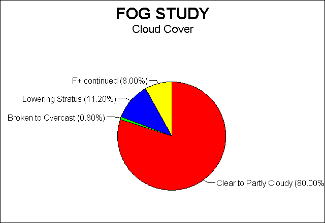
Figure 1.

Figure 2.
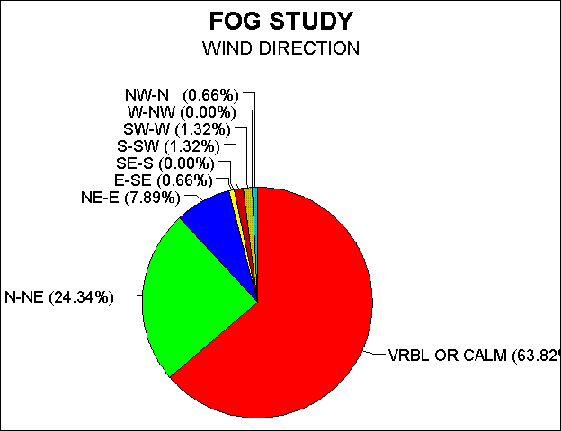
Figure 3.
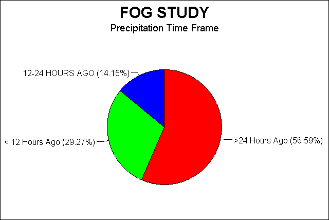
Figure 4.

Figure 5.


 Local Radar
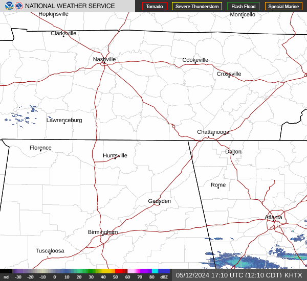 Huntsville Radar
 Regional Satellite
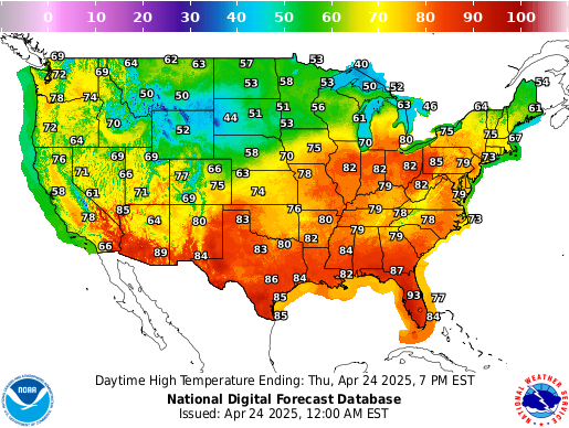 Graphical Forecast
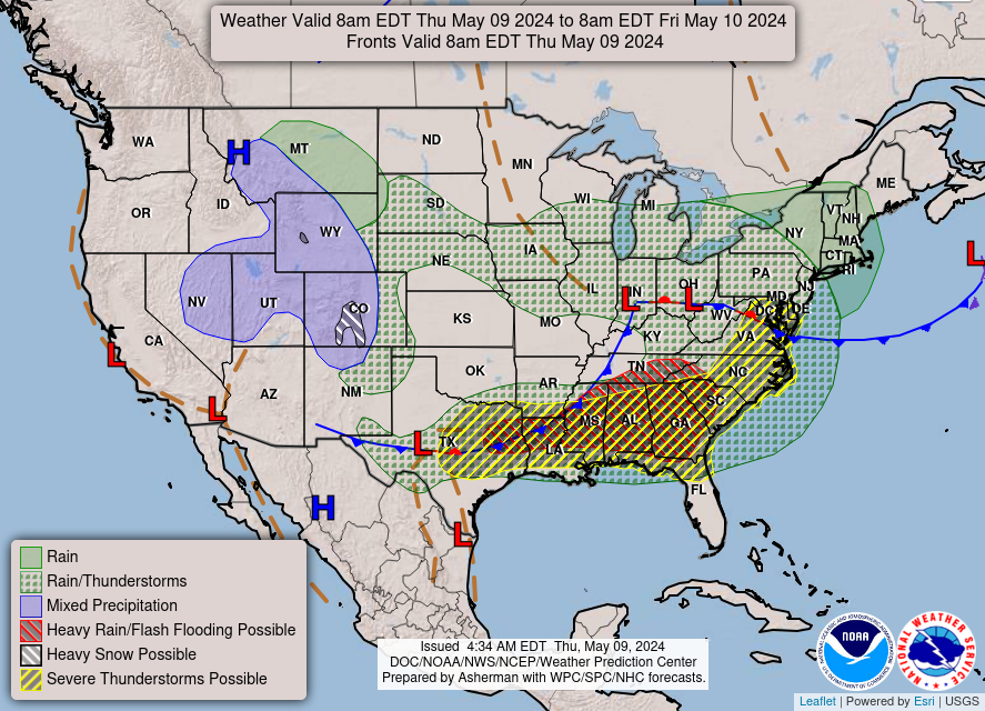 Weather Map
 Daily Graphics
 Follow us on YouTube