2013 Hollings Scholar Summer Project

Introduction

As part of the Ernest F. Hollings scholarship program, McKenna W. Stanford (University of South Alabama) spent much of the summer with the staff at WFO Springfield. David Gaede (Science and Operations Officer at WFO SGF) served as McKenna's mentor during his stay in Springfield. Jason Schaumann and John Gagan (Lead Forecasters at WFO SGF) both served as co-mentors to McKenna.

McKenna spent most of his time conducting statistical research of the three ingredients method presented by Schaumann and Przybylinski at the 2012 Conference on Severe Local Storms. McKenna's hard work and dedication have revealed very promising results regarding the three ingredients method for anticipating quasi-linear convective system (QLCS) mesovortex genesis and rapid intensification. The results of McKenna's work were presented to the WFO SGF staff, and were also presented to a diverse audience at the 2013 Student Science & Education Symposium in Washington, D.C. McKenna earned honorable mention for his presentation. Congratulations McKenna!

Methodology

The first step in this research was to search out potential QLCSs within a specified domain. We chose a domain which extended from the eastern Plains through the Midwest given the frequency of QLCS tornadoes throughout this region.

The search then began for QLCS cases within this domain for the 2005 to 2011 time period. In order to expedite the process, we initially sought out cases with the following criteria:

1. At least three reports of wind >= 58 mph or at least one tornado
2. Reports occurring within 50 nautical miles (nm) of an upper air (RAOB) site
3. Reports occurring within 50 nm of a radar site
4. Reports falling within 2 hours of synoptic RAOB times (00 UTC or 12 UTC)

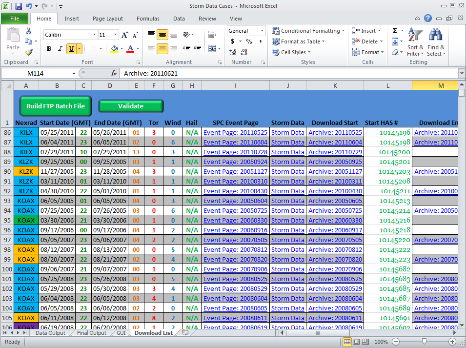
In order to expedite this process, Meteorological Intern Ryan Kardell wrote a series of scripts utilizing Microsoft Excel.  These scripts polled the National Climatic Data Center (NCDC) Storm Events Database via the Storm Prediction Center (SPC). A sample of the output from the SPC page can be found here.

Here are some screen shots of the user interface and output from Ryan's Excel program. Anyone interested in Ryan's scripts can contact him at Ryan.Kardell@noaa.gov.

After running Ryan's program, the search yielded roughly 200 potential cases. The next step in the process was for McKenna to inspect these cases and eliminate all non-QLCS cases. To accomplish this step, radar data was downloaded for all cases from the NCDC radar database. Inspection of hourly radar data from the Storm Prediction Center (SPC) mesoscale analysis archive in conjunction with the NCDC radar data resulted in a reduction of potential cases to around 90.

In order to properly test the statistical performance of the three ingredients method, we identified cases for placement into two separate "bins". The first bin contained known mesovortex cases. Our initial goal for this bin was to document approximately 50 mesovortices using 10 to 15 QLCS events. Given that QLCS events in this bin were known mesovortex producers, this bin would provide a good first test for the three ingredients method.

A second "random" bin was then defined with 20 cases selected for this bin. Cases for the random bin were selected with the following guidelines:

1. Select 10 cases where 0-3 km bulk shear was >= 30 knots
2. Select 10 cases where 0-3 km bulk shear was less than 30 knots

Of the 10 cases where 0-3 km bulk shear exceeded 30 knots, we intentionally selected five cases where the line-normal component of 0-3 km bulk shear appeared to be poor. The goal of this approach was to show the statistical significance of line-normal bulk shear versus straight-up bulk shear. Furthermore, the overall intent of the random bin was to test the three ingredients method in widely differing 0-3 km shear regimes to further show its utility.

Additional guidelines were then used to make the final case selections.

1. Select cases from varying radar and RAOB sites
2. Select cases from both the warm and cold seasons (We defined warm season as April through September and cold season as October through March)
3. Select cases where QLCSs vary in size

After careful consideration using the guidelines defined above, the following cases were selected for the "mesovortex" and "random" bins. Light red shading represents warm season cases while light blue shading represents cold season cases. The radar site and date is listed for each case.

Radar data for each one of these cases was then interrogated to document all occurrences of mesovortices and surges. All mesovortices and surges were then logged into a Microsoft Excel spreadsheet.

Gibson Ridge radar software (GR2Analyst) was used to interrogate the radar data. Storm relative motion (SRM), velocity (V), and reflectivity (Z) products were the primary products used to inspect for mesovortices and surges.

All mesovortices and surges had to meet the following criteria:

1. Occur within 40 nm of a RAOB site
2. Occur within 40 nm of a radar site
3. Occur within 2 hours of synoptic RAOB times (00 UTC or 12 UTC)

We only logged these features within 40 nm of both the radar and RAOB sites to ensure that the radar was not overshooting the genesis level of a typical mesovortex. Trapp et al. 1999 (hereafter T99) showed that mesovortex genesis occurs on average about one kilometer above ground level. As is often the case, mesovortices can grow upward with time and can subsequently be viewed at further distances from the radar.

In addition to the general criteria above, we also applied more stringent criteria to document both mesovortices and surges.

Mesovortices (all criteria below must be met)

1. The mesovortex persisted for at least two volume scans
2. Rotational velocities were >= 20 knots
3. The mesovortex reached at least 8000 feet in depth 

Surges

A surge was logged when the apex (bow structure) became displaced from the original updraft/downdraft convergence zone (UDCZ) >= 4 nm. Other visual cues were also used to identify potential surges including:

1. Radar animations indicated a clear forward acceleration which resulted in a concave (bowing) appearance to a line segment
2. The presence of a rear inflow notch (RIN)

An example of a surge is depicted within the cyan ovals below. This surge is approximately 30 nm west-northwest of the Huntsville, AL (KHTX) radar on 27 April 2011. The left frame depicts storm relative motion while the right frame depicts radar reflectivities. A mesovortex did develop north of this surge apex and persisted for several volume scans. Please note that this surge and mesovortex were not included in the database as they were not in close enough proximity to a RAOB site.

For every documented mesovortex and surge, 0-3 km bulk shear and line-normal bulk shear magnitudes were then computed. Hourly RUC model initialization data was used when available, with SPC mesoscale analysis and RAOB data used when RUC data was not available. Custom RUC 4-panel images were used to assess precise vector orientations and magnitudes for each mesovortex and surge. An example of one of these 4-panels is included below.

We would like to thank Dr. Chad Gravelle for the development of these 4-panel images!

You will notice in the 4-panel image that the standard 0-3 km bulk shear vectors are shown in the upper-left image when magnitudes are >= 30 knots. Meanwhile, the lower-left panel contains the vector magnitudes (knots) while the lower-right panel contains the orientation (degrees). All three of these panels display the vectors/values at grid point spacing of roughly 40 km.

Of particular note is the upper-right panel. This panel depicts the RUC model's depiction of ongoing precipitation at that initialization time. This precipitation graphic was vital in selecting uncontaminated values/magnitudes of ambient 0-3 km bulk shear. We intentionally sought out areas ahead of the model depicted precipitation. Often times, vector orientations and magnitudes will differ (become "contaminated") within areas of model generated precipitation.

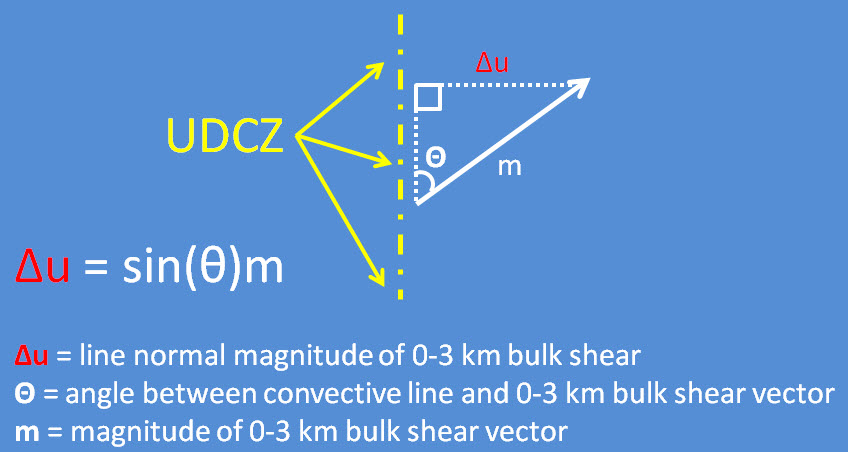
Line-normal magnitudes of 0-3 km bulk shear were then calculated for each mesovortex and surge. As is emphasized in Schaumann and Przybylinski 2012 (hereafter S&P12), line-normal 0-3 km bulk shear magnitudes are preferred to assess the amount of horizontal vorticity available to interact with QLCS cold pools. The line-normal component is critical given that individual line segments within QLCSs often exhibit differing orientations.

To derive line-normal magnitude, the angle between the 0-3 km bulk shear vector and the orientation of the UDCZ was computed. For mesovortices, we used the orientation of the UDCZ in the vicinity of the mesovortex at the time of mesovortex genesis. For surges, we used the UDCZ orientation immediately north of the surge apex. We chose this location given that most conceptual models depict the region immediately poleward or "left" of the surge apex as being the most favored area for cyclonic mesovortex genesis. Additionally, numerous formal case studies document the area immediately left of the apex as a favored area for mesovortex development. An example of the orientation of the UDCZ for a developing surge is included below.

Note that this line segment was eventually responsible for the 13 October 2012 Willard, MO tornado. A case study on this event can be found here. Please note that the Willard tornado case was not a part of McKenna's research as it fell outside of the 2005-2011 time frame.

Once the angle between the 0-3 km bulk shear vectors and UDCZ was known, we then used simple trigonometry to calculate the line-normal component of 0-3 km bulk shear:

In addition to the shear calculations for each mesovortex and surge, the shear/cold pool balance regime in the vicinity of these features was also logged. Shear/cold pool balance regimes were classified into one of five possible categories:

1. Shear dominant (SD)
2. Slightly shear dominant (SSD)
3. Balanced (B)
4. Slightly cold pool dominant (SCD)
5. Cold pool dominant (CD)

The shear/cold pool balance regime was primarily determined by comparing the UDCZ in the radar velocity data to the reflectivity field. Radar cross sections were also utilized to assess the vertical orientation and depth of updrafts. Listed below are common characteristics of the five shear/cold pool balance regimes.

 Shear Dominant

1. Near-surface UDCZ is located well behind developing updrafts
2. Radar cross-sections or all-tilts indicates updrafts are forward leaning with less vertical development
3. Width of the updrafts can be notably thin
4. Leading stratiform precipitation likely

1. UDCZ embedded within or immediately behind vigorous convection
2. Radar cross-sections or all-tilts indicates updrafts are slightly forward leaning and fairly deep in nature (often not as deep as balanced region)
3. Often contain a thin area of leading stratiform precipitation but also contain an expansive area of trailing stratiform precipitation

1. UDCZ located immediately downstream of vigorous convection
2. Radar cross-sections or all-tilts indicates updrafts are nearly vertical and deep in nature (perhaps compared to other convection within the QLCS)
3. A strong reflectivity gradient is noted on the forward flank of the segment
4. Echo tops are higher than surrounding convection
5. Trailing stratiform precipitation

1. UDCZ (gust front) is slightly ahead of the main convection (by 3 or more nm)
2. Radar cross-sections or all-tilts indicates updrafts are slightly rearward leaning and fairly deep in nature (often not as deep as balanced region)
3. Trailing stratiform precipitation

1. UDCZ (gust front) is clearly outrunning the main convection
2. Radar cross-sections or all-tilts indicates updrafts are leaning rearward with less vertical development
3. Trailing stratiform precipitation

Below is a set of images which depicts a line segment containing three of the five shear/cold pool balance regimes. These images depict an expanded view of the line segment which spawned the Willard, MO tornado on 13 October 2012. Storm relative motion is depicted in the left image while radar reflectivities are depicted in the right image. RAP40 0-3 km bulk shear vectors are overlaid in black. 

Several other data calculations and tabulations were logged into the Excel spreadsheet for each mesovortex and surge.  
Here is a list of what was logged for each of these features:

• Date
• RDA
• County
• Nearest city/town
• Upper air (RAOB) site
• Mesovort ID number (if applicable)
• Surge ID number (if applicable)
• Time of mesovort genesis (if applicable)
• Was a surge present? (Y/N)
• Time of surge genesis (if applicable)
• Time of first tornado report (if applicable)
• Time of first wind report >= 58 mph (if applicable)
• Other storm reports (if applicable)
• Is the mesovort at least 8000 feet deep? (Y/N)
• Surge/mesovort UDCZ orientation (degrees)
• 0-3 km bulk shear vector orientation (degrees)
• 0-3 km bulk shear vector magnitude (knots)
• Line-normal 0-3 km bulk shear magnitude (knots)
• Shear/cold pool balance regime (SD/SSD/B/SCD/CD) 
• Surge to mesovort lead time (if applicable)
• Mesovort to wind damage lead time (if applicable)
• Mesovort to tornado lead time (if applicable)
• Surge to tornado lead time (if applicable)

Click on the images in the table below to view screen shots of the Excel database. 

Results

After tabulating results for both the mesovortex and random bins, a total of 67 mesovortices were identified. All mesovortices were associated with a surge. A total of 64 non-mesovortex surges were also identified.

52% of the 67 identified mesovortices produced at least one report of winds >= 58 mph and/or a tornado.

31 of the mesovortices produced at least one wind report, while 21 produced at least one confirmed tornado.

Please note that only the first wind damage and tornado report associated with a mesovortex was counted. Several of the mesovortices did go on to produce additional wind reports and/or tornadoes.

Statistical verification of the three ingredients method was as follows:

• The probability of detection (POD) was 79%
• The false alarm rate (FAR) was 23%
• The critical success index (CSI) was 64%

Recall that the three ingredients method dictates that mesovortex genesis and strong intensification is favored when ALL THREE of the following criteria are met:

1. A portion of a QLCS exhibits a nearly balanced or slightly shear dominant shear/cold pool balance regime
2. 0-3 km line-normal bulk shear magnitudes are equal to or greater than 30 knots
3. A rear-inflow jet (RIJ) or enhanced outflow causes a surge or bow in the line

One important point we want to emphasize when computing the statistical performance of the three ingredients method is that we used whole numbers for the 0-3 km line-normal magnitudes. We simply rounded to the nearest single digit. Interestingly, operational meteorologists using vectors (wind barbs) to assess shear magnitudes encounter even less in the way of precision as these barbs are typically displayed in five knot increments. With rounding also in play, a 30 knot shear vector could represent shear values anywhere from 27.5 knots up to 32.4 knots. For the sake of this research, we felt that rounding to the nearest whole number represented a sound compromise.

In contrast, shear magnitudes deduced from statistical plots below are listed to the nearest tenth. We felt this increased precision would allow us to better present statistical analysis of the shear magnitudes.

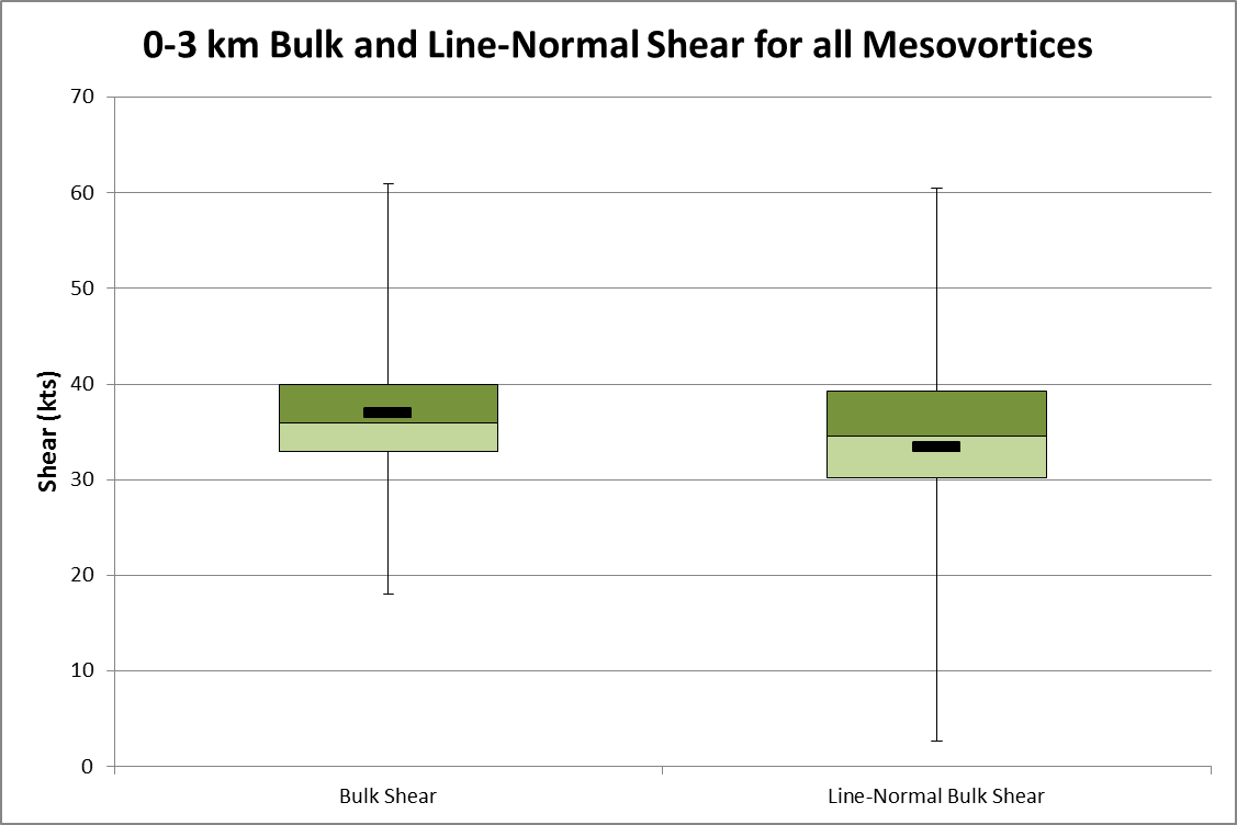
In the box-and-whisker plot below, the mean 0-3 km bulk shear magnitude for mesovortices was 37.3 knots while the mean line-normal bulk shear magnitude was 33.5 knots. The lower quartile line-normal shear magnitude for mesovortices was 30.2 knots.

This next plot depicts 0-3 km line-normal bulk shear magnitudes for both mesovortex, and non-mesovortex surges. As was established in the first plot, the mean line-normal magnitude for mesovortices was 33.5 knots. The mean value for non-mesovortex surges was 25.9 knots.

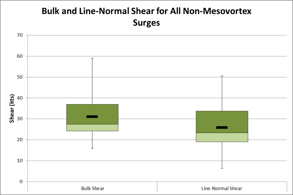
The following plot depicts 0-3 km bulk and line-normal bulk shear magnitudes for all non-mesovortex surges. The mean magnitude for bulk shear was 31.0 knots. As was established in the previous plot, the mean line-normal magnitude for non-mesovortex surges was 25.9 knots.

The next set of graphics below depicts 0-3 km bulk shear and line-normal bulk shear magnitudes for wind reports (first graphic) and tornadoes. Please note that from this point forward, all wind report graphics and statistics depict reports of >= 58 mph winds associated with mesovortices only. We counted a wind report as being associated with a mesovortex if it occurred within 5 nm of an identified mesovortex.

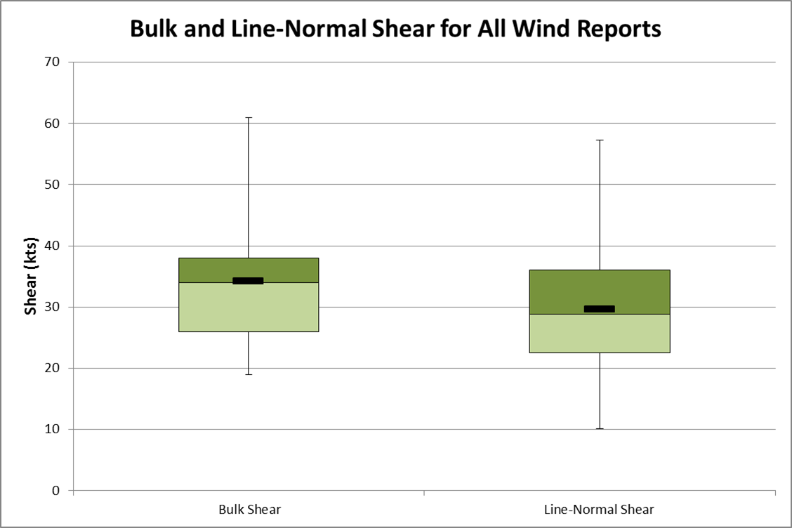
The mean bulk shear value for wind reports was 34.2 knots while the mean value for tornado reports was 36.9 knots. The line-normal values for wind versus tornado reports showed a bit more separation. The mean value for wind reports was 29.7 knots while the mean value for tornado reports was at 34.5 knots. The lower quartile line-normal magnitude for tornado reports was 31.0 knots.

McKenna's work also revealed some other noteworthy statistics:

• The average surge genesis to mesovortex lead time was 9 minutes
• The average lead time from mesovortex genesis to the first report of wind damage was 14 minutes
• The average lead time from mesovortex genesis to the first tornado report was 10 minutes

Perhaps the most revealing statistics were as follows:

• The average lead time from surge genesis to the first report of wind damage was 21 minutes
• The average lead time from surge genesis to the first report of a tornado was 18 minutes

McKenna then ran statistics on one final scenario. If a Tornado Warning was issued every time the three ingredients criteria were met, what would the statistics reveal? One strong word of caution here...we are not advocating that warning decision makers (WDMs) should issue a Tornado Warning every time the three ingredients criteria are met! We simply ran these statistics as a litmus test...a "what if" scenario. The results were as follows:

• The POD was 86%
• The FAR was 74%
• Average lead time was 18 minutes

While the FAR is certainly high in nature, let's compare these statistics to the 2013 National Weather Service (NWS) Government Performance Requirements Act (GPRA) goals for Tornado Warnings:

• POD = 72%
• FAR = 70%
• Average lead time = 13 minutes

When comparing the two sets of statistics, the three ingredients method offered a 14% increase in POD and a 5 minute increase in lead time. It did result in a slightly poorer FAR. Interestingly, NWS lead times for Tornado Warnings are often much higher for tornadoes produced by supercell thunderstorms versus those from QLCS mesovortices. In other words, Tornado Warning lead times for QLCSs often fall short of the 13 minute GPRA goal.

Discussion and Summary

Examination of the first two box-and-whisker plots reveals that the mean line-normal magnitudes for mesovortex(non-mesovortex) surges were 33.5(25.9), respectively. The lower quartile value for mesovortex surges was 30.2 knots. Thus, 75% of logged mesovortices had line-normal magnitudes at or above 30.2 knots. There also appears to be a considerable amount of separation between the mesovortex and non-mesovortex surge plots. There is a slight area of overlap in the 30.2 to 33.8 range, with the latter number representing the upper quartile magnitude for non-mesovortex surges. Finally, the p-value for line-normal shear magnitudes when comparing mesovortex and non-mesovortex surges was significantly lower than 1%. This indicates a high level of statistical significance and is supportive of the 30 knot line-normal 0-3 km bulk shear magnitude threshold presented by S&P12.

Inspection of the third box-and-whisker plot reveals the importance of the line-normal component of 0-3 km bulk shear. The plot for bulk shear straddles the 30 knot threshold with a mean value of 31.0 knots. The upper quartile for bulk shear was 37.0 knots while the lower quartile was 24.3 knots. In contrast, the line-normal shear plot indicates a majority of data points fell below the 30 knot threshold. The mean magnitude for the line-normal plot was 25.9 knots with an upper quartile value of 33.8 knots. The p-value for all non-mesovortex surges when comparing bulk shear and line-normal bulk shear magnitudes was well below 1%. This indicates strong statistical significance supporting the utility of the line-normal magnitude of 0-3 km bulk shear.

The final two box-and-whisker plots also reveal some noteworthy statistics. The vast majority of tornado reports occurred with 0-3 km bulk shear magnitudes greater than 30 knots with the lower quartile magnitude for this plot at 33.5 knots. Meanwhile, line-normal magnitudes for tornado reports featured a lower quartile value of 31.0 knots. While the plots for wind reports showed considerable overlap with those of the tornado reports, one can deduce that both bulk shear and line-normal bulk shear magnitudes >= 30 knots support an increased likelihood for mesovortex tornadoes.

Using the 30 knot threshold, forecasters may then use 0-3 km bulk shear vectors to anticipate mesovortex potential in advance. While line-normal magnitudes cannot be computed before the development of a QLCS, forecasted 0-3 km bulk shear vectors can be used as a starting point. If a QLCS is anticipated, comparing 0-3 km bulk shear vectors to its expected track and orientation may reveal the potential for mesovortex development. This potential could then be conveyed in outlook products, web briefings, etc.

Perhaps the greatest utility of the three ingredients method is in warning operations. One of the most common methods for issuing Severe Thunderstorm and Tornado Warnings for QLCS mesovortices is to issue the warning AFTER the mesovortex develops. As the results of this research have shown, the average duration between mesovortex genesis and the first wind(tornado) report was 14(10) minutes, respectively. T99 showed that the "lead time" between mesovortex genesis and the first tornado may actually be as little as 5 minutes. Thus, WDMs waiting for mesovortex genesis to occur before issuing a warning often results in warnings with little in the way of lead time.

Utilizing the three ingredients method offers WDMs multiple advantages in support of more advanced and accurate warnings. First off, this methodology gives WDMs a step-by-step process by which to interrogate QLCSs for potential mesovortex genesis. This process is outlined below.

Radar Interrogation and Time Budget during a QLCS Event

1. Monitor 0-3 km bulk shear vectors in the ambient atmosphere ahead of the QLCS and determine what UDCZ orientations would result in line-normal magnitudes >= 30 knots.
   • Time interval: Every 30 minutes or when new SPC mesoscale analysis/RAP data becomes available
   • When: During high radar tilts
2. Identify differing shear/cold pool balance regimes along the QLCS. Seek out balanced and slightly shear dominant regimes. Pay attention to the evolution of these regimes!
   • Time interval: Every 2-3 radar volume scans
   • When: During high radar tilts
3. Monitor for developing and ongoing line surges/bows. Use animations! Look for other clues such as rear-inflow notches.
   • Time interval: Every volume scan
   • When: Entire volume scan
   • Tip: If meeting criteria for items 1 and 2 above, ready a polygon when a developing surge is detected!
4. Monitor for developing and persisting mesovortices (in conjunction with surge/bow interrogation).
   • Time interval: Every volume scan
   • When: Low to possibly mid-level radar tilts

Using this outlined strategy keeps WDMs ahead of the game rather than having to quickly react to "surprise" mesovortices. Tracking 0-3 km line-normal bulk shear magnitudes almost become an afterthought. Very little time and effort is needed to keep tabs on this ingredient. Meanwhile, the tracking of shear/cold pool balance regimes does not require intense and constant interrogation since regimes evolve with time. Thus, WDMs can spend most of their time interrogating for developing surges/bows.

While the three ingredients method offers WDMs a system to manage the complexities of QLCS radar interrogation, it also offers additional advantages for warning accuracy and lead time. As was shown above, practicing this method effectively hones in on favored areas for mesovortex genesis. Doing so effectively eliminates large portions of QLCSs where mesovortices would not be favored. This would support more accurate warnings through effective polygon placement. Additionally, WDMs that ready polygons upon the genesis of a surge (assuming the other two ingredients are present) would stand to gain at least a few minutes of lead time. At the very least, the development of a surge should lead radar operators to increase situational awareness in that area of the parent QLCS.

Future Work

Our next goal is to complete formal research and publish a journal article on the three ingredients method. This research would include expansion of the dataset utilizing radar sites which are not collocated with RAOB sites. We may also explore the statistical significance of other environmental parameters such as low level CAPE. Finally, we may tie in the presence of other radar signatures such as reflectivity tags, rear-inflow notches, and front-end nubs/notches.

One other item we will be watching for closely is the presence of tornado debris signatures (TDSs). Since the installation of dual polarization radar, we have documented several occurrences of TDSs with the Springfield radar. Given that most mesovortex tornadoes are rain-wrapped in nature (not visible), it is quite possible that they are underreported. The presence of dual pol TDSs may reveal that greater frequencies of mesovortex tornadoes are occurring.

Acknowledgements

First off, we would like to thank McKenna for his hard work and dedication during the summer of 2013! McKenna's contributions to this project were nothing short of exemplary.

We would also like to thank Ryan Kardell for his Excel programming wizardry and his assistance in calculating statistical results.

We are also greatly in debt to Dr. Chad Gravelle for his fine work in generating the RUC 4-panel images. Chad's affiliations are listed below:

• • GOES-R Satellite Liaison - NWS Operations Proving Ground
  • CIMMS/SSEC University of Wisconsin - Madison
  • NOAA/NWS Training Center