OHD/HL - Threshold Runoff: User Doc: Functionality

2.2.1 Overview
2.2.2 Main Functions

2.2 Functionality

2.2.1 Overview

Given the database described in Section 2.1, an experienced ArcView user could manually estimate threshold runoff for a single basin in a relatively short period of time (~ 1 hour).  Most of this could be done using standard "off-the-shelf" ArcView and Spatial Analyst functions.  The challenge, however, is to automate parameter estimation procedures so that threshold runoff calculations can be made on thousands of basins at once without requiring an extensive knowledge of ArcView.  This is the purpose of the ArcView threshold runoff software (AV-ThreshR).

AV-ThreshR  is developed using Avenue, the customization and development programming language that comes with ArcView.  Avenue is a powerful, high-level language that allows quick and flexible automation of many spatial and tabular operations and quick user interface development.  Avenue programs are stored in documents called Scripts.  During development, Avenue scripts are saved in an ArcView Project file along with information about the customized GUI and data Themes of interest.  For distribution, this customized environment is saved as an ArcView Extension file (threshr.avx) so that users can load all of the AV-ThreshR tools and GUI elements into their own existing projects.  Using an Extension, all of the Avenue programs can be delivered in a single ASCII file.  An external C++ program is called from within Avenue to derive network connectivity.  The compiled C++ code is also delivered with the ThreshR software.  This external code is used because the equivalent Avenue code is much slower; however, the equivalent Avenue code is also included in the Extension for users who want a platform independent version of AV-ThreshR.

Two Menus, "ThreshR" and "ThreshR-Utility", are added to the default ArcView View GUI when the ThreshR extension is loaded. Customized tools have also been added to the Tool bar.  For the simplest and most straightforward implementation, the end-user is only concerned with items under the "ThreshR" menu.  The "ThreshR-Utility" menu contains programs used for data preparation and pre-processing; however, these programs are not needed to calculate threshold runoff and are provided for the advanced user only.  This document describes the programs underneath the "ThreshR" menu.  Items under the "ThreshR-Utility" Menu and the Tools added to the ToolBar will be described in other documents.

2.2.2.  Main Functions

The general approach used to calculate gridded threshold runoff is fairly simple:  define a set of subbasins, calculate topographic and climatic subbasin characteristics, use regression equations to compute the 2-year or 5-year return period peak flows for each subbasin (use Q2 or Q5 as a surrogate for bankfull flow), compute the unit hydrograph peak flow for each subbasin, compute threshold runoff for each subbasin, and interpolate subbasin threshold runoff values to the HRAP grid for use in the gridded Flash Flood Guidance software.

A summary of important outputs from AV-ThreshR  is provided here.

• Shapefiles of subbasin boundaries, outlet points, stream lines, subbasin center points and longest flow path lines are created.  The Shapefile of subbasin boundaries will contain thousands of basins in each RFC.  The user has control over the size of the analysis area and how many subbasins are created.

 
• Topographic and climatic parameter values required for empirical unit graph equations and USGS flood frequency equations (USGS WRIR 94-4002) are computed and stored in the subbasin boundary attribute table.  Some basic subbasin characteristics are computed in all locations while other (state specific) parameters are computed only where needed for the USGS regression equations.  A summary of the basic parameters computed by AV-ThreshR at all locations is provided in in Table 2.2.1.  The names of the output fields used to store the parameters in the subbasin value attribute table are also provided.  The letter "L" preceding the field name signifies a "local" (as opposed to cumulative) parameter.  For non-headwater basins, local and cumulative parameter values differ.  For many parameters, it is most efficient to first compute local parameters for all subbasins and then compute cumulative parameter values as a function of local parameters.  More details about parameter calculations methods are provided below in the Compute Subbasin Parameters section.

• Threshold runoff is computed at the outlet of each delineated subbasin and values are interpolated to the HRAP grid.

• An ASCII file of threshold runoff values that can be read by the Flash Flood Guidance program is exported.

 

Items in the main "ThreshR" pull-down menu are shown in Table 2.2.2.  The ThreshR menu items are divided into logical groups that are color coded in Table 2.2.2 (separated by a horizontal bar in the actual software).  Steps 2, 3, and 4 are pure GIS processing steps.  Step 4, "Compute Subbasin Parameters," is the most time consuming step (taking 32.5 hours for 9000 subbasins in MBRFC (the largest RFC)).  Time estimates for Steps 2 and 4 are roughly 21 minutes and 2 minutes respectively.  These time estimates are highly system dependent.  The relatively long time required for calculations in Step 4 is not overly burdensome when using a 400-m DEM and relatively large subbasins (9000 subbasins covering MBRFC); however, computation time will become a bigger issue if it is proven that using much smaller subbasins provide significantly improved results (on the order of 10 times more  subbasins were used in GRASS ThreshR trials and at least 10 times more subbasins will be produced in the NSSL National Basin Delineation project).  For reasons discussed in the Compute Subbasin Parameters section, deriving two parameters in particular significantly increase the computation time (slope of the longest flow path (CHSL) and length to the point on the longest flow path opposite the subbasin centroid (CHCN)).  Alternative computational methods that could substantially reduce the computation times for these parameters are discussed.

Upon initially delivery of AV-ThreshR, a first pass of Steps 2, 3, and 4 will already be completed.  A user may want to repeat these processing steps at a later time (e.g. using higher resolution DEM data).  Steps 4 and 5 require the user to make some hydrologic judgements appropriate for their local areas (e.g. choosing to use Q2 or Q5 as a surrogate for bankfull flow or specifying Snyder Unit Graph parameters).  However, with all the complex parameter calculations completed in Step 4, these programs run relatively fast (a few minutes for an entire RFC).  Therefore, the user may easily repeat these steps using different options to derive the most satisfactory results.  A detailed description of the user options, computational methods, inputs, and outputs of each of the steps listed in Table 2.2.2 is provided below.

Table 2.2.2 Main ThreshR Menu
 

ThreshR --> Setup

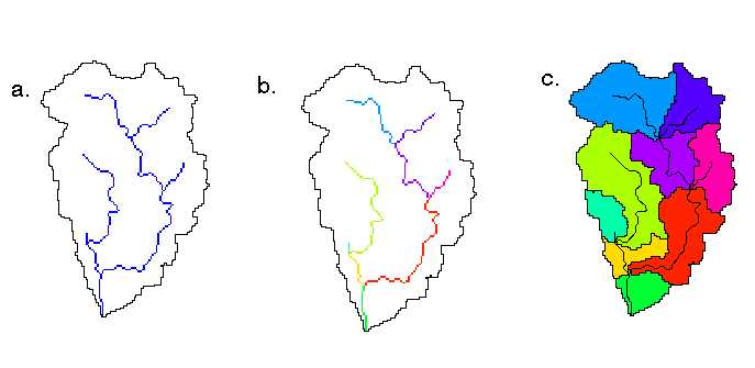
Function: The setup script serves two purposes:  (1) allows the user to specify the directory location of the input data, and (2) automatically loads data Themes from the user specified location into the active View.

User Interface/Options:  An input box appears which allows the user to type the directory location of the input data.  Following this input box, the user may choose whether or not to proceed with loading the input data (Yes or No).  If the answer is Yes, the following Themes are added to the active View: regions.shp, rf1.shp, rfcbound.shp, statekey.shp, hrappts.shp, slopeff, fld, mask, fa, fd, and dem.  A description of each of these data Themes is provided in Table 2.1.  In addition to these Themes, two data tables containing parameter information and regression equation coefficients are added to the Project.  Use of these tables is described later in this document.

Notes:  As explained in the Tutorial, the output directory for the project should be set before running Setup.  To do this, make the Project window active and then select Project --> Properties.  In the "Project Properties" window enter the name of the desired output directory in the "Work Directory" text box.  It is also a good idea to set the View map and distance units to meters.  To do this:  With your View active, click View --> Properties and set map units to meters and distance units to meters and click OK.

ThreshR --> Define Subbasins

Function:  Define subbasin boundaries from the flow direction Grid.

Method:  AV-ThreshR uses a sequence of standard ESRI hydrologic functions to delineate basin boundaries.  The required inputs for subbasin boundary definition are the flow direction and flow accumulation grids described in Section 2.1.3.2.  Given the flow accumulation Grid, a stream network is defined by assigning all cells with a flow accumulation greater than a user defined area threshold the value one and assigning all other cells the value NODATA Figure 2.2.1a.  The cells in each distinct reach of the resulting stream network are assigned a unique grid code (stream links) (Figure 2.2.1b) and a network of subbasins is defined by assigning all cells that drain to a given reach the same grid code (Figure 2.2.1c).

Figure 2.2.1 (a) gridded streams defined using a 60 km2 threshold, (b) stream links, (c) subbasins.

For the example shown in Figure 2.2.1, the area threshold used to define streams is 60 km2.  This means that the drainage areas at the tips of the streams is 60 km2 and the smallest possible size for a headwater subbasin is equal to the area threshold.  The sizes of the resulting subbasins are not uniform; some are small and some are large (this is no different from the GRASS version of threshR).  In this example, a 1409 km2 area is divided into 9 polygons with an average area of 156.6 km2, a minimum area of 67.4 km2, and a maximum area of 292 km2.   The average area of the 4 headwater basins is 180 km2, nearly 3 times the stream threshold.  If a lower stream threshold is chosen, more subbasins are created as shown in Figure 2.2.2.  In this case, the average are of 10 headwater basins is 65.5 km2, compared with a stream threshold of 30 km2.  For thousands of headwater basins delineated in ABRFC and MBRFC using stream thresholds of 30 km2 and 60 km2, the average headwater basin sizes were about a factor of 2.3 times the stream threshold used.
 

Figure 2.2.2  21 Subbasins with 10 headwater basins.  Headwater basins average area is 65.5 km2 when a 30 km2 threshold is used to define streams.

For threshold runoff calculations, the objective of subbasin definition is to create a sampling of outlet points covering a large geographic area where computations can be made; therefore, the stream threshold based algorithm for defining subbasins is adequate.  There may be drawbacks to this approach for other applications.  For modeling applications, the sizes of the basins created might not be desirable.  It might be of interest to combine several small subbasins into one or divide a long subbasin into two parts.  Although this type of functionality can be provided within the ArcView environment, it is not required to derive gridded threshold runoff estimates and tools to accomplish such tasks are not included in the initial threshr.avx extension.  Some other basic delineation tools are included in threshr.avx, but these tools are not part of the base AV-ThreshR functionality.  Tools for delineating a subbasin based on a single point clicked with the mouse or based on many points defined in a file are available provided.  These tools are simply customized versions of other tools that are widely used in the hydrologic engineering community.

Vector Shapefiles of the stream lines (strc1.shp), Shapefiles of the subbasin boundaries (shd1.shp), and a Shapefile of subbasin outlet points (outc1.shp) are created in this step using ESRI raster to vector conversion functions.  These files, along with the stream grid (1's and 0's) (strg1) and subbasin boundary grid (shdgri1) are saved for later use and added to the active View.  Output files are written to the Project working directory.  Upon creation, the first part of the names for each of these themes is fixed (strc, shd, outc, strg, and shdgri).  The trailing integer in each of the file names is incremented if the program is run multiple times in the same working directory.  Theme names can be modified by the user if desired.

The attributes "Area" and "Perimeter" are added to the shd1.shp file and the attributes "From_node" and "To_node" (used for determining connectivity in the next step) are added to the strc1.shp (Figure 2.2.3).  The polygons and stream lines that correspond to the same subbasin share the same Gridcode.

Figure 2.2.3  Subbasin Polygon and Stream Line Attribute Tables

The Gridcodes in shd1.shp and strc1.shp are also the same as the "Value" field in the shdgri1 Value Attribute Table (VAT).  During raster to vector conversion (using the Avenue AsPolygonFtab request), it is possible that a cell (or string of cells) that does not share a side with other cells of the same Gridcode (they are diagonally connected), may be created as separate polygons.  These polygons are referred to as dangling polygons.  Allowing these dangling polygons to persist might cause problems because the number of records in the subbasin polygon attribute table would differ from the the number of records in the subbasin Grid Value Attribute Table.  Therefore, dangling polygons are eliminated in shd1.shp by merging dangling polygons with bigger polygons that share the same Gridcode.

User Interface/Options:  The Subbasin Definition Dialog allows the user to do the following:

• Specify the drainage area threshold (km2) used to define the smallest headwater basin.

 
• Edit the default names for the flow direction and flow accumulation grids supplied by the program.  For standard runs, the program will provide the correct names for these Themes.  This option is only provided for users who want to skip around in the processing sequence.

 
• Specify that the area to be analyzed should be restricted to the area of a specified polygon Theme ("Analyze Only Selected Area").

 
• Specify a drainage area limit above which subbasins will not be delineated.  The default area suggested is 2000 km2 because this is often stated as the largest basin to which unit hydrograph theory can be applied.  Subsequent threshold runoff calculations can procede whether or not a subbasin threshold is used in the basin definition step.  The user may choose to delineate basins of all sizes (no drainage area limit), but restrict threshold runoff calculations to small basins in a later step.

Inputs: flow direction grid, flow accumulation grid

Outputs:  A polygon subbasin boundary Shapefile (shd1.shp), a line stream file (strc1.shp), a point subbasin outlet file (outc1.shp), the stream grid (1's and NODATA), and the subbasin Grid (shdgri1) are added to the active View.
 

ThreshR --> Determine Connectivity

Function:  Determine the connectivity among subbasins.

Method:  In order to calculate subbasin parameters like drainage area, longest flowpath, mean annual precipitation, etc. required for regression equations, the connectivity of subbasins must be known.  This is because the flow at point 3 (Figure 2.2.4) depends not only on the intervening or "local" area between the junction of subbasins 1 and 2 and point 3 but on all of the upstream area ("cumulative" area).  The exact way in which the connectivity information is used to calculate parameter values varies for different parameters.  This is discussed further in the next section.

Figure 2.2.4 Local area and cumulative area examples.

The connectivity between subbasins is known based on the "From_node" and "To_node" attribute fields added to the stream line attribute table (strc1.dbf).  Using this information, the record numbers for all subbasins upstream of each basin are computed and stored.  This information is stored so that the upstream connectivity only needs to be computed once.  The program used to identify upstream subbasins ("IdUpstream") is modeled after a program written by Zichuan Ye (now a consultant at ESRI).  The original code was written in Avenue, but has been translated into C++ here for improved speed.  The tracing algorithm uses a "Stack" object.  Although the user need not be concerned about the inner workings of these codes, it is helpful to identify the intermediate and final information that gets generated.

For easier access from an external program, the From_node and To_node information is exported from the stream shapefile (strc1.dbf) to an ASCII file.  This intermediate file is named the same as the corresponding subbasin shapefile with a different extension (".gtf") (e.g. shd1.gtf) and written to the same location as all other output (the Project working directory).  The IdUpstream program creates another intermediate file containing information about the sequence in which the tracing of subbasins occurs.  This file is saved with an ".ord" extension (e.g. shd1.ord).  From the "ord" (order) file, the file of most interest, a file with the ".ups" extension, (e.g. shd1.ups) is also created.  The shd1.ups file contains one line for each subbasin in shd1.shp that is not a headwater.  Each of these lines contains the record number for a subbasin followed by a list of record numbers for all upstream subbasins.  The record numbers are used here rather than the Gridcode integer values because this considerably speeds up processing in the subbasin parameter calculation algorithms.  This is not a problem as long as a user does not manually delete or add any records to the subbasin Shapefile.  If this occurs, then the connectivity algorithm must be rerun.

User Interface/Options:  The Determine Connectivity dialog allows the user to do the following:
 

• Edit the default names for the subbasin and stream line Themes supplied by the program.  For standard runs, the program will provide the correct names for these Themes.  This option is only provided for users who want to skip around in the processing sequence.

• Choose not to use the external C++ program for determining basin connectivity.  This option is irrelevant for RFC users because the compiled C++ program will be delivered with the software.  The option to use the original (less efficient) Avenue codes for determining connectivity are included for users without a C++ compiler.

Outputs:  3 ASCII files: shd1.gtf, shd1.ord, and shd1.ups.  The fields "shdishead" and "shdisout" are added to shd1.shp.
 

ThreshR --> Compute Subbasin Parameters

Function:   All required topographic and climatic parameters are computed for each subbasin.

Methods:

The methods for parameter calculations are best described using an example.  All 24 parameters required for USGS flood flow regression equations in MBRFC are described in Table 2.2.3.  A discussion how these parameters and any additional basic parameters listed in Table 2.2.1 is provided below.

Table 3.3 Example Parameter Code Table (parcode.dbf) for MBRFC

Table 2.2.3 contains the same information as a table called "parcode.dbf"that is used by the software to (1) define the fields used to store calculated results, (2) identify the source data for making parameter calculations, and (3) identify any unit conversions that are required.  This data table is customized for each RFC to reflect the parameters required by the USGS flood frequency equations.  In this way, different parameters are computed where necessary, without having to modify  the Avenue code.  The file format used for this data table is dBase.  Considering ArcView capabilities, the three most practical choices for the format of this file were ASCII, dBase, and INFO.  The dBase format was chosen over the INFO format because it is more portable.  Initially, comma delimited ASCII files were used for this file because dBase files have a limitation on field name length (10 characters) which makes it more difficult to convey the meaning of each data field.  However, it is very convenient to be able to edit table entries in parcode.dbf (and regequat.dbf described below) through the ArcView interface.  This can't be done for ASCII files so a switch to the dBase format was made.  In future versions of AV-ThreshR, one way to get around the dBase field naming limitations would be to use field Alias names within ArcView.

For MBRFC, fields to contain all the parameters listed in Table 2.2.3 are added to the subbasin attribute table (shd1.dbf).  The field names added to shd1.dbf are identical to the parameter codes ("Parcode") listed in Table 2.2.3.  The type, display width, and display precision for these fields are specified using the values in the "Ftype," "Fwidth," and "Fprecision."  A brief description of each parameter ("Descrip") and the units ("units") required for the regression equations are also given in Table 2.2.3, but this information is not used by the Avenue codes.  "Meastype" is a key word indicating to the program what type of routine is required to make the calculation.  In MBRFC, there are only two options: basic and basin_average.  The key word "basic" actually covers several types of parameter calculations as described below.  The field "Srcfile" contains the file name of a Grid or Shapefile that is required to make the parameter calculation.  An "x" entry indicates that no source file is required for this particular parameter.  Basic parameters do not require source files.  Parameters calculated as a function of one of the basic parameters listed in Table 2.2.1 also do not require source files.  The "Srcdir" field indicates whether or not the source data file is located in the input file directory specified in Step 1 (indicated by an "x" in Table 2.2.3) or in a subdirectory of this input file directory.  The "Srctype" field indicates what type of data is required to compute the parameter value.  If the parameter is computed from a data file, the source type is either "grid" or "poly."  If the parameter is computed based on information in another parameter field, the name of that parameter field is given.

The "Conversion" field indicates whether or not a units conversion and/or adjustment factor needs to be applied to the source data to calculate the parameter value in a manner consistent with the regression equations described in USGS Report 94-4002.  The codes "a","s","m", and "d" are used to indicate add, subtract, multiply and divide respectively.  If one of these ASCII codes is used, a number indicating a multiplicative or additive factor must follow the code, with an underscore separating the code and the factor.  Multiple operations can be made for the same parameter by separating operations with an underscore.  This type of conversion is used when computing parameters such as mean basin elevation in New Mexico (ELV_NM) which must be in units of thousands of feet.  The vertical units of the digital elevation model (DEM) obtained from NOHRSC are meters.  It is not efficient to store the entire DEM in all conceivable units; therefore, mean basin elevation values are computed in meters and then converted to the desired units.   The string "m_3.281_d_1000" in the Conversion field for ELV_NM indicates that the mean subbasin elevation in meters should be multiplied by 3.281 and divided by 1000 to get units of thousands of ft.

basin average parameters
21 of the 24 parameters listed in Table 2.2.3 are simply basin averages.  For headwater subbasins, these averages are computed in one of three ways depending on the "Srctype:"  (1) For grids, the result is simply an average of the values of all cells within the subbasin (when the resolution of the grid of interest like mean annual rainfall is coarser than the DEM resolution, the average is for all of the cells that intersect or are completely within the subbasin, (2) for polygons, the result is an average of the values associated with all of the polygons that intersect the subbasin weighted by the fraction of area covered by the pieces of these polygons within the subbasin, and (3) if the Srctype is the name of a field like "lelvmean" (local mean elevation), the parameter value is simply this value, with perhaps a unit conversion or adjustment factor applied.  Spatial averaging Grid or polygon values within a zone (subbasin) are common GIS applications illustrated in Figure 2.2.5.

Figure 2.2.5 (a) grid zonal (subbasin) mean and (b) polygon area weighted averages

Both gridded and polygon data are allowed as source data for AV-ThreshR parameter calculations because some data types are more appropriately represented as rasters while other data types are more appropriately represented using a vector format.  Continuously varying data such as rainfall are most easily represented using a raster format, but discrete data sets (like soils and water bodies) are often more efficiently and accurately stored in a vector format.  The philosophy in developing the AV-ThreshR database and software was to leave source data in their original format whenever possible.

Computation of basin averages for non-headwater subbasins is more complicated and involves two steps.  The first step is to compute local subbasin parameters and the next step is to compute cumulative values by taking a wieghted average of the values in the upstream areas.  For gridded value data (e.g. mean annual rainfall), computing statistics for thousands of local subbasins is very efficient because a standard function (or request) designed for this task can be called within Avenue.  The results of the zonal (subbasin) average calculation are copied to the subbasin attribute table (shd1.dbf) for later use in computing cumulative parameter values.  As seen in Table 2.2.1, several statistics related to local elevation, slope, flow length, and flow accumulation are computed and stored in the subbasin attribute table.  With this information, the algorithm to compute cumulative basin averages is to loop through each subbasin, and if it is a non-headwater, select the records of all upstream subbasins and compute an area weighted average value.  Upstream records are selected using information in the file "shd1.ups" described in the last section.  A database object called a Bitmap in Avenue allows efficient selection of records from large attribute tables.

stateabbr, regions, and reg_fract

If a basin intersects more than one state, the location of the basin centroid is used to determine which flood flow regression equations will be used.  Areas outside the state of interest are ignored when spatial averages of parameters (like SLPM_KS) only known inside the state of interest are computed.  For subbasins that intersect more than one regression equation region in a given state, it is necessary to determine the fractional area of the subbasin in each region.  This requires the cumulative subbasin shape (polygon) for non-headwaters, not just the local shape.  For each non-headwater, the local shapes of all selected upstream records are merged to form the cumulative shape.  The centroid of the cumulative shape is also determined.  Centroid points for all subbasins are saved in a Shapefile called cntp1.shp.  The state containing the basin centroid is also determined and saved in the "stateabbr" attribute field of shd1.shp.  A list of regions intersected by the cumulative subbasin shape is stored in the "regions" field and the corresponding fractions of the cumulative shape in each region is stored in the "reg_fract" field.

CHLN, CHSL, CHSL0, and CHCN

There are a several parameters of interest for which the derivation is more complicated than computing a straight subbasin average.  These parameters are channel length, channel slope, and length to a point on the channel opposite the channel centroid.  The need to compute these parameters raises the question: What is a channel?  Digital line maps showing the locations of streams such as EPA's RF1 and RF3 files contain some guidance as to the locations of known "channels;" however, several difficulties arise in using these data sets to define channels.  On difficulty that arises is that there is a huge difference in the stream detail provided with these two data sets.  Many small basins defined using AV-ThreshR will contain no RF1 streams but many RF3 streams.  RF3 files and the new (National Hydrography Dataset)NHD data set are certainly more accurate than RF1, but these datasets are too large to use nationally in the first AV-ThreshR release.  Even with the capacity to deal with RF3 or NHD, there are limitations as to the consistency of how streams are defined because the stream mapping techniques used to create these files are often subjective, and different scale source maps were used to build the digitial RF3 in some parts of the country.  Fortunately, in developing the flood flow regression equations, the USGS uses a standard method for measuring "channel" length and slope which does not require a precise definition of where the actual channel begins (USGS WRIR 86-4335; USGS WRIR 87-4008).  The channel length (CHLN) used in the regression equations is more accurately described as the length of the longest flow path or the length from the subbasin outlet to the furthest upstream point on the basin divide.  The slope of the longest flow path (CHSL) is defined as the difference in elevation between points 85% and 10% along the longest flow path divided by the length between these two points.

The length to a point on the main channel opposite the channel centroid (CHCN) is of interest because Snyder (1938) chose to use this parameter in a regression equation for computing lag.  Carpenter and Georgakakos (1993) used a regression relationship developed by Gray (1961) to relate CHCN to channel length (CHLN), rather than actually computing CHCN.  The regression equationship given by Gray shows that CHCN is highly correlated with  CHLN, which makes one wonder whether both of these variables are needed in an expression for the basin lag time.  The strategy adopted for AV-ThreshR is to go ahead and calculate the CHCN parameter, but maintain flexibility so that this relatively expensive parameter computation can be avoided (if necessary) when higher resolution DEM data are used.

Given the CHCN and CHLN values computed with the existing database, regional empirical relationships between CHCN and CHLN could be easily derived and used to estimate CHCN when higher resolution DEM data are used.  Figure 2.2.6 shows such a relationship that was derived for ABRFC.  A similar strategy might also be necessary to reduce computation time for CHSL as explained later.  An Avenue script that works on vector objects is used to calculate CHCN given the longest flow path shape (discussed below) and the basin centroid point (See Figure 2.2.8).

Figure 2.2.6  Empirical elationship between the CHCN and CHLN parameters for ABRFC.

Computationally, there is a significant difference between determining only the length of the longest flowpath and actually creating a line representing the longest flowpath.  Creating the line representing the longest flow path provides an easy mechanism for calculating the CHCN and CHSL parameter values.  This computational expense is not significant when considering only a single basin, but becomes important when calculations are made for thousands of basins at once, as required to derive gridded threshold runoff estimates.  The algorithm used to create a vector line representing the longest flowpath in a headwater basin is as follows:
 

1. Identify cells within the basin that have the longest flow length by querying the flow length grid (in some cases, multiple grid cells on the basin divide may have equally long flow lengths so one of these points is arbitrarily selected).
2. Trace the path from the farthest cell to the subbasin outlet using the flow direction grid.
3. Convert the gridded flow path trace to a vector line object for later use.

Figure 2.2.7  Example of longest flowpath shapefile.

Using the longest flowpath line segment, the longest flow path slope (CHSL) is determined by identifying points at 85% and 10% away from the outlet and extracting the DEM values from underneath these points (Figure 2.2.8).  This is the primary method used for calculating "channel" slope in AV-ThreshR because this is the slope measurement method used by the USGS when deriving regression relationships.  A second, much more efficient method for calculating longest path slope is also used.  The field name used to store the results for this parameter is CHSL0.  CHSL0 is computed as the difference between the maximum subbasin elevation along the longest flowpath (lemaxlfp) and the minimum subbasin elevation (lelvmin), divided by the longest flow path length.  When calculations are made for subbasin 9, the lemaxlfp value is from furthest upstream subbasin (i.e. subbasin 1) and lelvmin is from the local subbasin 9 area.  For a given subbasin, computing slope using these two methods can produce significantly different results.  CHSL0 (100%-0%) is typically higher than CHSL (85%-10%) because elevation-distance curves tend to be steeper in the top 15% of a basin.  For 3506 subbasins in ABRFC, the average value of CHSL0 is 38.1 ft/mile and the average value of CHSL is 30.9 ft/mile.  In the future, when a higher resolution DEM and many more subbasins will be used (See Future Plans), having a more efficient algorithm for computing CHSL is desirable.  An alternative to developing a more efficient algorithm for CHSL would be to use regional relationships like that shown in Figure 2.2.9 to predict CHSL from CHSL0, a parameter that can be computed much more quickly with existing algorithms.

Note:  It is not correct to compute the longest path slope by simply averaging the values of all corresponding cells in the slope grid slopeff (See Table 2.1 for definition of this grid).  This method of calculation gives an unrealistically high "channel" slope estimates because the average slope of a 400 m grid cell does not reflect the actual slope of the stream bed (or even the actual location of the stream).  In the Figure 2.2.8 example, the slope calculated using this method would be 405 ft/mile -- much higher than the correct value of 16.4 ft/mile.

Figure 2.2.8  Computing CHSL for subbasin 9.

Figure 2.2.9 Empirical elationship between the CHSL and CHSL0 parameters for ABRFC.

Controlling which parameters actually get computed for a given location

The parcode.dbf table contains information about each parameter that needs to be computed, but it does not control whether a given parameter is actually computed for a given subbasin.  This is because some parameters, such as SLPM_KS (soil permeability in Kansas), only need to be computed for subbasins in specific states.  In fact, it it would be impossible to compute this particular parameter for all states in the RFC because the soil permeability data layer called slpm_ks.shp only covers the state of Kansas.  Records in the shd1.dbf table that do not represent subbasins with their centroids in Kansas will not have an entry for the SLPM_KS field.  An attribute called "params" in the statekey.shp Theme tells the program which parameters need to be computed for a given state.  The "params" attribute field does not include parameters listed in Table 2.2.1.  Parameters listed in Table 2.2.1 are basic parameters that get computed at all locations.

User Interface/Options:  The Compute Subbasin Parameters dialog allows the user to do the following:
 

• Edit the default names for input Themes supplied by the program.  For standard runs, the program will provide the correct names for these Themes.  This option is only provided for users who want to skip around in the processing sequence.

 
• Choose to calculate "All Parameters," "Basic Parameters Only," or "USGS Regression Parameters Only."  If the "Basic Parameters Only" option is selected, the user may choose to "Customize" parameters calculations.  If this option is selected, the user is prompted to select parameters of interest from a list.  For a base run, a user would normally choose "All Parameters."  Including some flexibility in parameter calculation choices has been important in the development phase because it helps with debugging.  Flexibility will also be important in the implementation phase under certain scenarios -- if, for example, the USGS regression equations for an area get updated and require additional parameters.  A user may choose to customize basic parameter calculations so that expensive parameters such as CHSL and CHCN are not computed (As discussed above, CHSL and CHCN can subsequently be estimated using regression relationships.) or some users may wish to calculate the basic parameters for purposes other than computing threshold runoff.  Warning:  Customizing "Basic Parameter Calculations" may prohibit using the "USGS Regression Parameters Only" option at a later time.

• Choose maximum subbasin size for which parameter calculations will be made.

Outputs:  Multiple parameter fields are added to subbasin polygon attribute table.  Fields required for a given subbasin location are populated with data.  A longest flow path Shapefiles (Lfp1.shp) and a center point Shapefile (cntpt1.shp) are created.

ThreshR --> Compute Q2, Q5, etc.

Function:

Calculate return period flood flows in all subbasins of interest for a selected return period.

Methods:

All states intersecting the analysis area are selected.  A loop is made through these selected states.  All of the equation information from the file regequat.dbf for the currently selected state is temporarily read into memory.  Regequat.dbf contains coefficient and exponent information required to calculate peakflows in each state and USGS region.  For each subbasin with its centroid in the currently selected state, flood flow calculations are made.  Parameter values obtained from the subbasin value attribute table (shd1.dbf) are used to evaluate the regression equations.  When a subbasin intersects multiple regions, an area weighted average of the return flows is computed using information in the fields "regions" and "region_fract" of shd1.dbf.

An example of the regression equation information in regequat.dbf for Wyoming is shown in Table 2.2.4.

Table 2.2.4 Example of Regression Equation Table entries (regequat.dbf) for Wyoming

In Table 2.2.4, the "regionnum" in regequat.dbf is identical to the "reg_num" in regions.shp.  "Arealevel" is used only if there are different equations specified for basins of different sizes (e.g. Colorado Plains Region).  The "Special" field contains zero if the regression equation conforms to a the standard format shown in Equation 1.  A unique integer code is entered in the "Special" field for any state/region combinations that do not conform to the standard multiple regression format in Equation 1.  For example, a 2 indicates to the program that an alternative equation in which the first independent variable is raised to a quantity equal to a constant times itself raised to a constant (Equation 2).  The regression equation format with the Special code 2  is applicable to the Wyoming Plains and High Desert regions as well as all of Kansas and Missouri.

Equation 1    Q = a*(X^b)*(Y^c) . . .

Equation 2    Q = a*(X^(b*X^c))*Y^d*Z^e . . .

The "numterms" field stores the number of independent variables in the regression equation and the "terms" field stores a string containing the parameter codes (also the parameter field names in shd1.dbf).  Each entry in the "terms" field is separated by a vertical bar "|".  The "coeffs" field contains strings specifying the regression equation coefficients and exponents.  In the coefficients string, each value is also separated by a vertical bar "|".

User Interface/Options:  The  USGS Flood Frequency Calculation dialog allows the user to do the following:
 

• Edit the default names for input Themes supplied by the program.  For standard runs, the program will provide the correct names for these Themes.  This option is only provided for advanced users who want to skip around in the processing sequence.

 
• Select the return period of interest from a pulldown box (2, 5, 10, 25, 50, or 100 years).  In some states and regions, the regression equations for all of the return periods listed may not be available in USGS WRIR 94-4002.  If this is the case, a flag of -1 is entered in the output field.

• Enter a string to uniquely identify this run.  This is used to determine the names of the output field.

Inputs:  Subbasin theme, analysis area theme, statekey.shp

Outputs: A field containing the peak flow value for the user selected return period is added to the subbasin shapefile(s).  The units for the output field are cfs and the output field is named Qn_x by default where n is the return period and x is the run identifier.  If a field by this name already exists, the user is prompted to choose another identifier or delete the existing field manually.

ThreshR --> UG Peak Flow

Function:

Calculate unit graph peak flow using Snyder's method for 1 hr, 3 hr, and 6 hr durations.

Methods:

Using the basin characteristics ARM, CHLN, and CHCN from shd1.dbf and equations from Snyder (1938), the peak flows for a 1 hr, 3 hr, and 6 hr duration are estimated for each subbasin.  The Ct and Cp Snyder parameters are either entered in an input box by the user or specified using a polygon Shapefile.  If Ct and Cp are entered through the input box, the same parameters are used for all subbasins.  If a polygon Shapefile is used, then spatially distributed Ct and Cp values can be specified.

Time to peak for the standard unit graph is computed as

Equation 3   tp=Ct*((CHLN*CHCN)^0.3)  'time to peak in hours

The standard Snyder duration (tr) is estimated.

Equation 4   tr=tp/5.5

The time to peak corresponding to the duration of interest (tpR) is computed.  tR is the duration of interest (1, 3, and 6 hours)

Equation 5   tpR=tp-((tr-tR)/4)

The peak flow for the duration of interest (qpR) is calculated.

Equation 6   qpR=640*Cp/tpR   'required unit graph peak in cfs/(in*mi2)

User Interface/Options:  The  Unit Graph Peak Flow dialog allows the user to do the following:
 

• Edit the default names for input Themes supplied by the program.  For standard runs, the program will provide the correct names for these Themes.  This option is only provided for advanced users who want to skip around in the processing sequence.

 
• Select the unit hydrograph method from a pull-down menu.  The only method available in the initial release is the Snyder method.

 
• Check the box "UG Parameters from a File" if you want to specify unit hydrograph parameters using a Shapefile or Arc/Info coverage.  If this box is checked, a "UG Parameter Theme" input text line appears where the user can enter the name of the UG parameter Theme.  To use this option, the selected Shapefile must have Snyder coefficients stored in attribute fields called "Cp" and "Ct."  For each subbasin where calculations are made, the Cp and Ct values that fall beneath the center point of the subbasin are used in unit graph peak flow calculations.

 
• If "UG Parameters from a File" is not selected, the user is prompted to enter Cp and Ct values for the analysis area.

• Enter a string to uniquely identify this run.  This is used to determine the names of the output fields.

Inputs: subbasin Theme, center point Theme (optional)

Outputs: Fields "Qsd1_x," "Qsd3_x," and "Qsd6_x" with units of cfs are added to the subbasin attribute table.  These fields containt the 1 hr, 3 hr, and 6 hr unit hydrograph peak estimates respectively.  x is the run identifier.
 

3.2.7  ThreshR --> Subbasin Threshold Runoff

Function:  Calculate the threshold runoff for selected durations.

Methods:
This function simply provides a user interface for dividing the bankfull flow values by the unit hydrograph peak values to derive threshold runoff.  If either of the input estimates is less than or equal to 0, then the output value is set to -1.

User Interface/Options:  The  Subbasin Threshold Runoff dialog consists of two pulldown boxes and a list box.  A user should first "Select Subbasin Theme" (first box).  When this is done, the "Select Bankfull Flow Field" box and "Select UG Peak Flow Field" list box are automatically updated.  A user can select an appropriate bankfull flow field (e.g. Q2_1) and an appropriate unit graph peak flow field (e.g. Qpsnyd1hr) using these boxes.  The user is prompted to enter the name of the output field that will be created by the program (e.g. tr1hr).  The user is notified if a field with this name already exists,

Inputs: User specified bankfull flow and unit hydrograph fields.

Outputs: An output field containing the threshold runoff estimate for a specific duration.

3.2.8  ThreshR --> Interpolate to HRAP
 

Methods:  Computed threshold runoff values are assumed to apply to the intervening area between the calculation point and the next upstream subbasin outlet.  The values assigned to these intervening areas (polygons) are mapped to HRAP center points (hrappts.shp).  An inverse distance weighting interpolation scheme is used to create a continuous threshold runoff grid that covers all areas, even gaps where threshold runoff was not computed due to the maximum area threshold specification (e.g. 2000 km2).  The interpolated values are mapped to all HRAP center points in the region.

User Interface/Options:  The Interpolate to HRAP dialog allows the user to edit the default names for input Themes supplied by the program.  For standard runs, the program will provide the correct names for these Themes.  This option is only provided for advanced users who want to skip around in the processing sequence.

Inputs:  hrappts.shp, threshold runoff field in shd1.shp

Outputs:  a field containing threshold runoff values is added to hrappts.shp

3.2.9  ThreshR --> Write FFG ASCII File

Function:  From the threshold runoff values stored in hrappts.shp, create an ASCII file that can be read by the FFG program.

Inputs: hrappts.shp

Output: ASCII file