OHD/HL - GIS: Training Workshop

Introduction:

Part of the reason that ArcView is such a powerful tool is that custom applications can be built using the Avenue language.  Unfortunately, this also means that ArcView functionality can be packaged in many different ways, which may be confusing to a new user.  Several raster analysis functions useful for basin definition and hydrologic parameter estimation are available with the Spatial Analyst (e.g. the flow direction, flowaccumulation, and watershed functions).  Because these functions are not accessible through the standard Spatial Analyst GUI, many customized ArcView extensions have been developed to assist non-Avenue programmers with basin boundary definition and parameter estimation.

Tools developed by ESRI are generic tool kits:

• Hydrologic Modeling (v. 1.0)
• Hydrologic Modeling (v. 1.1)

• AV-ThreshR (1999-2000)  (NWS-HRL)
• AMBER Basin Delineation (NWS)
• HEC-GeoHMS (ESRI, HEC) -- This combines features from
• HECPrepro (Univ. of Texas at Austin) and
• Watershed Delineator (ESRI, TNRCC)

Requirements:

Software:  ArcView v. 3.1 or later and Spatial Analyst v. 1.1 or later.

User Knowledge:

• It is assumed that the user has a basic knowledge of ArcView terminology and knows how to navigate the ArcView user interface. For those people used to running Windows software, learning ArcView is fairly intuitive. For users that have little or no ArcView experience, it is STRONGLY RECOMMENDED that you go through the ArcView "Quick Start Tutorial" Chapter 2, Exercise 1 in the book "Using ArcView" that is distributed with the software, and the Spatial Analyst "Quick Start Tutorial," Chapter 2 in "Using the ArcView Spatial Analyst," also distributed with the software. Learning the basics of ArcView will only take a few hours and can be fun. Files for these tutorials can be found on the installation CDs. [At HRL, files for the ArcView tutorial are located on the NHDRs in the directory /nonawips/gis/avtutor/arcview. Files for the Spatial Analyst tutorial are located in the directory /nonawips/opt/arcview3/avtutor/spatial.]

Input data for this workshop have been pre-installed in a directory called "tkdata" on the student workstations.

Workshop Instructions

2. Create a new directory for output files in your workspace and then specify this directory as the project Working Directory by clicking on Project --> Properties with the Project window active.  Type the name of your output directory in the space next to "Work Directory" and click OK.

3. Open a new View and click  to load the DEM called "springdp" from the "tkdata" directory.  Note: To see a list of grid themes on your hard disk, you need to select "Grid Data Source" as the "Data Source Type" in the Add Theme window.  Make the springdp Theme visible and your View should look similar to the one shown here.

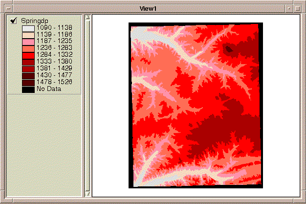
This is a DEM covering the 7.5 minute quadrangle called Springdale, Arkansas.  This DEM was obtained via anonymous ftp to a webserver at the USGS Eros Data center.  These data are distributed in the UTM projection but the data have been reprojected and resampled into an Albers Equal-Area projection so that the data can be displayed with other data sets used in this workshop.  Make "springdp" the Active Theme by clicking the mouse on the text "springdp" in the View Table of Contents and then click Theme --> Properties to get information about this Theme.
 

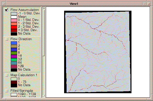
What is the cell size for this grid?
How many rows and columns are there?
What area does the grid cover?

5. Click Hydro --> Fill.  This may take a few minutes depending on the speed of your computer.  This program creates a "hydrologic" DEM by filling sinks (or pits) in the landscape.  A sink is a cell or group of cells surrounded on all sides by cells of higher elevation.  Sinks are often present in DEMs due to sampling effects during DEM creation.  Sinks created due to the sampling method are artificial and therefore should be removed.  The fill function removes sinks in the DEM by raising the elevations of sink cells to the minimum height that would allow water trapped in the sink to flow out.  Some DEM sinks are real inland drainage areas and should not be filled; however, methods to identify real sinks and include these in a basin data set are beyond the scope of this workshop.

6. (Optional -- Advanced Legend Editing Exercise) See where the DEM was filled.  Click Analysis --> Map Calculator.  In the "Map Calculation 1" window, double-click on [Filled Springdp], click on "-", and then double click on [springdp] to create a grid that is the difference between these two inputs.  Click Evaluate to create a new grid called "Map Calculation 1."  Close the Map Calculation window by using the pulldown menu in the upper left corner of the window or typing Alt-F4.  Edit the legend for Map Calculation 1 so that all cells with nonzero values are a dark-solid color and all the zero cells are displayed with transparent fill.  This can be done by setting the number of classification fields to 2, manually typing in the legend ranges to represent 0 and non-zero values, and then editing the symbol for zero values to be transparent.  By doing this, you will see that most of the filled cells are located in valley botoms where channels whould normally be.  This makes sense because artificial sinks are more likely to occur in channel areas where an elevation sample at the bottom of a channel will appear as a sink relative to surrounding cells sampled in the overbank area.

7.  Make "Filled Springdp" the active Theme (by clicking on the TEXT "Filled Springdp" in the Table of Contents) and click Hydro --> Flow Direction.  A Flow Direction Grid is created in which each cell is assigned an integer code indicating which flow direction is assigned to that cell.  The algorithm used to assign flow directions is the D8 model. Codes are as follows: (1 = East, 2 = Southeast, 4 = South, 8 = Southwest, 16 = West, 32 = Northwest, 64 = North, 128 = Northeast).   Place a check mark next to the "Flow Direction" Theme and this gives you a preview of where the drainage patterns lie.  Make Flow Direction the Active Theme and click  to see the attribute table for the Flow Direction Grid.  Which direction is the most popular among all the cells in the Flow Direction Grid?  Select a row in the "Attributes of Flow Direction" table and you will see the corresponding cells highlighted in your View.  Select Edit --> Select None if you wish to remove this selection.  Close the Table window.  

8.  Make sure "Flow Direction" is still the active Theme and click Hydro --> Flow accumulation.  In the "Flow Accumulation" grid that gets created, cells are assigned a number corresponding to how many DEM cells are upstream.   Double-click on the Flow Accumulation Theme to edit its legend.  Click "Classify" to change the classification "Type" from "Equal Interval" to "Standard Deviation."  Click OK and then click Apply.  (You can close the Legend Editor window using Alt-F4).  Using this classification scheme reveals a drainage network of cells containing high flow accumulation values.   With the Flow Accumulation Theme active, Zoom In   closely to an area with drainage paths and query the values  of flow accumulation stream cells above and below stream junctions.  By doing this, you can see how the drainage areas sum correctly when a tributary enters a main river.  Zoom back to the full extent  before continuing.

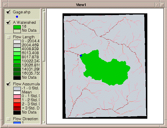
9.  Make Flow Direction the active theme and click Hydro --> Flow Length.  Click "Yes" to calculate length to an outlet.  Each cell in the Flow Length grid contains an estimate of the length (m) from each cell to the nearest outlet.  In this case, outlets are the edge of the DEM.  We will come back to the Flow Length grid later in this workshop.

10.  Select Hydro --> Properties.  Enter "Flow Direction" as the Flow Direction Theme and "Flow Accumulation" as the Flow Accumulation Theme and Click OK.  By doing this, you have now made the tools  and   accessible (Previously they were "grayed-out").

11.  The  tool (sometimes called the "Raindrop" tool) can be used to trace the flow path from any point on the DEM to the edge of the DEM.  Turn off (remove check marks next to) all Themes except the "springdp" DEM.  Click  and then click a point on the DEM.  Click additional points as you wish.  This tracing tool creates graphics in the View window (not Themes).  To remove these graphics, select Edit --> Select All Graphics and then Edit --> Delete Graphics.

12.  Now delineate a basin draining to a selected outlet grid cell.  From the "tkdata" directory, load a point Theme called gage.shp.  Set "Data Source Type" to "Feature Data Source" in the Add Theme Dialog to see a list of Shapefiles on the hard disk.  Place a check mark next to this Theme and you will see a point in the western portion of this example area.  This is not a real stream gage location, but let's pretend this is a stream gage above which a basin boundary is needed.  Make the Flow Accumulation Theme (with the Standard Deviation legend classification) visible underneath the gage point and you will see that this point falls close to the drainage network defined by the DEM.

13.  Make the Flow Direction Grid Theme active, and click on the  tool and then on the gage point to delineate a basin.  You may want to zoom in closer to make the selection easier.  The point you select does not have to fall directly on the drainage network defined by the DEM.  Rather than selecting the DEM cell immediately under the point clicked by the mouse, the  tool in the Hydrologic Modeling Extension v. 1.0 chooses the cell within 240 m of the point clicked that has the highest flow accumulation as the watershed pour point.  Thus, the mouse-selected point is actually snapped to the river network.  This snapping can be somewhat annoying as it is often desirable to zoom in and choose a specific cell for your outlet.  This snapping can easily be changed using Avenue -- a similar watershed delineation tool available in the AV-ThreshR extension does not force this arbitrary snapping distance.

The Grid Theme "A Watershed" is added to your View by this tool.  Turn this Theme on to see the delineated boundary.  You should see something similar to what is shown below.

Note:  The grid code assigned to your watershed may be a number other than 16.

It is a good idea to save your project at this point File --> Save Project As ( I have had an inexplicable crash on an HP machine if the charting option is selected in the next and last step.)

14.  Calculate Flow Length statistics for this watershed.  Make "A Watershed" the active Theme and select Analysis --> Summarize Zones. When prompted, pick Flow Length as the theme containing the varialbe to summarize and click OK.  Select Cancel when asked to select a statistic to chart since it is pretty useless to chart a single value.  You should see a table that shows Min, Max, Mean, and other statistics for the Flow Length values that fall within this watershed.  The length of the longest flow path in the watershed is simply the Max value minus the Min value.  Units are Meters.  This is an example of one type of calculation that is done in AV-ThreshR to estimate the longest flow path length parameter that is used in unit graph calculations.