Meteorological Processes in the Atmosphere (Part 2)
FRONTOGENESIS
- Frontogenesis is a very important and common atmospheric process that refers to a change in the magnitude and orientation of a thermal (temperature) gradient at a level or in a layer due to horizontal changes in the total wind (i.e., due to patterns of convergence and divergence). This change (i.e., frontogenetical forcing) alters thermal wind balance, which forces a vertical motion response in the atmosphere which can result in mesoscale bands of enhanced precipitation.
- Frontogenesis = an intensification of a temperature gradient at the surface or aloft.
Frontolysis = a weakening of the gradient.
- During frontogenesis, a thermally direct circulation is produced which is on a smaller scale (lower end of the meso-alpha scale) than the direct circulation associated with the entrance region of a jet streak. In low levels, rising motion usually occurs near the warm side of the low-level temperature gradient (i.e., slightly displaced from the maximum frontogenesis area). The ascent causes adiabatic cooling. Parcels eventually exhibit weaker sinking and adiabatic warming well on the cool side of the low-level thermal gradient.
- Frontogenetical zones often slope upward toward cold air. Thus, the vertical component of the circulation will be sloped with height toward cold air as well (complements isentropic lift). The horizontal components of the frontogenetical circulation consist of an acceleration of air parcels from cold-to-warm air in low levels and from warm-to-cold air at upper levels. This circulation acts to weaken the thermal gradient that frontogenesis attempts to strengthen.
- The smaller-scale direct thermal circulation forced by frontogenesis usually enhances the larger-scale direct circulation in the entrance region of a jet streak, leading to an intensified and more focused mesoscale upward motion area (i.e., the two circulations act synergistically). Vertical motion values from frontogenesis can be on the order of 10s (roughly 20-40) of cm/s (versus 5-10 cm/s for jet dynamics/isentropic lift). In other words, significant frontogenesis can double or triple vertical motion values over a smaller-scale from that due to isentropic lift/warm advection on the synoptic-scale. Therefore, identifying frontogenetical areas is crucial, since it can result in a distinct band of heavy precipitation within surrounding lighter precipitation.
Q VECTORS/F VECTORS
- We can qualitatively assess frontogenesis by looking at surface and upper air charts of wind and temperature. However, frontogenetical forcing can be assessed more accurately and quantitatively by looking at "Q vectors" or "F (frontogenesis) vectors" (Fig. 1). Q and F vectors are not "real" winds, but they are used to describe how the geostrophic (Q vectors) or real wind (F vectors) changes the isotherm/thickness patterns that can lead to vertical motion.
 |
Fig. 1: Q vectors (or F vectors) in the natural coordinate system. Q is the total vector; Qn and Qs are those components of Q that are directed perpendicular and parallel to isotherms or thicknesses (solid lines), respectively. When Q points from cold to warm air (as shown at left), geostrophic frontogenesis is implied (see text for more details). |
- In theory, Q vectors (which assume use of the geostrophic wind) are related to vertical motion via the quasi-geostrophic omega equation. F vectors (which employ the total/actual wind) are not. The total wind can be broken into two components, the geostrophic (non-divergent part of the) wind and the ageostrophic (divergent part of the ) wind. By doing this, equations of motion and other meteorological equations can be developed to model flow patterns and various processes in the atmosphere. For the sake of proper theory, the following discussion will reference Q vectors, which are readily available in the NWS's Advanced Weather Interactive Processing System (AWIPS). However, it should be noted that F vectors (which can be added to the AWIPS Volume Browser) seem to correlate very well to locations of banded precipitation. Q vectors also typically show good overall correlation to banded precipitation patterns.
- The magnitude and direction of Q vectors describe how the magnitude and orientation of a thermal gradient are changing, and whether geostrophic frontogenesis or frontolysis is occurring. When Q vectors point from cold-to-warm (warm-to-cold) air in the low-and-middle levels of the atmosphere, geostrophic frontogenesis (frontolysis) is taking place (Fig. 1).
- Convergence of Q vectors often is associated with forcing for ascent, while divergence of Q typically is associated with descent.
- Q vectors can be broken down into two vector components (natural coordinates): Qs and Qn (Fig. 1). Qs is the rotational component of Q, and is directed parallel to isotherms/thicknesses. Qn is the frontogenetical component of Q, and is directed normal/perpendicular to the temperature lines.
- Qs vectors basically describe temperature advection patterns, and force vertical motion on the synoptic scale. Qs describes how the orientation of the isotherms/thicknesses is changing with time due to horizontal changes in the geostrophic wind. Qs vectors are most pronounced in areas where the wind is tending to rotate isotherms significantly, i.e., in areas of warm and cold advection. The longer the Qs vectors, the greater the temperature advection pattern and forcing for synoptic scale vertical motion. Typically, ahead of (behind) a storm system, Qs convergence (divergence) will be present, which represents forcing for ascent (descent) associated with warm (cold) air advection (Fig. 2). Forcing fields associated with Qs often are relatively broad and weaker than that for Qn.
 |
Fig. 2: Example of Qs vectors, Qs divergence (solid lines), and Qs convergence (dashed lines) in the 850-700 mb layer. Convergence is shown over the Ohio Valley where low-level warm advection (not shown) was occurring. Thus, this is an area of forcing for synoptic-scale ascent. Divergence over the Plains was coincident with cold advection, i.e., forcing for descent. |
- Qn vectors can be very important (the dominant term), and forces vertical motion on the mesoscale/frontal scale. Qn describes how the magnitude of the thermal gradient is changing, i.e., the gradient is becoming stronger (frontogenesis) via confluence or weaker (frontolysis) via difluence. Qn vectors are longest where the thermal gradient is changing the most, not necessarily where the tightest thermal gradient exists. Convergence of Qn vectors represents forcing for ascent; divergence of Qn forces descent (Fig. 3). Typically, Qn convergence fields (especially from 1000-700 mb) usually are linearly aligned and often associated with enhanced banded precipitation given sufficient moisture.
 |
Fig. 3: Example of Qn vectors, Qn divergence (solid lines), and Qn convergence (dashed lines) in the 850-700 mb layer. Qn pointed from cold to warm air indicating a frontogenetical situation. Strong convergence over Kentucky and Tennessee was forcing for significant frontogenetical forcing and ascent. This example is from the January 17, 1994 snowstorm over Kentucky, where 1 to 1.5 feet fell in a narrow axis in central Kentucky. Heavy snow was occurring at this time in central Kentucky. |
- Identifying frontogenetical areas, especially in the cool season, is very important, because these are areas where significant upward vertical motion and banded precipitation likely will be located, given adequate moisture and saturation. Qn vectors can be used to assess frontogenesis. The longer the Qn vectors, the greater is the geostrophic frontogenesis (i.e., Qn vectors are longest where the temperature gradient is strengthening the most), and the more the vertical motion response must be. Ascent in low-levels is near the warm side of the frontogenesis maximum with the frontogenetical zone and area of ascent usually tilted toward cold air aloft (Fig. 4).
 |
Fig. 4: Frontogenesis produces a mesoscale direct thermal circulation that is sloped with height toward cold air. Q/F vectors are longest where frontogenesis is the greatest. On the periphery of this area, Q/F vectors are shorter given weaker frontogenesis. Thus, Q/F vector convergence (forcing for lift) occurs on the southern/eastern periphery of the maximum frontogenesis area (as shown at left). A steeply sloped frontogenetical zone in low-to-middle levels can produce a definitive band of heavy precipitation (rain or snow) superimposed on broader, lighter precipitation in cool season. In the warm season, low-level frontogenesis also can force the lift needed to promote deep convective development and subsequent heavy rainfall. |
- Qn vectors should be evaluated in the 1000-850 mb layer when boundary layer convergence/forcing is occurring or expected (e.g., along/near surface/low-level cold fronts, or possibly during convective situations when boundary layer forcing is vital). In isentropic lift/overrunning situations, 850-700 mb layer Qn vectors (e.g., Figs 2 and 3) should be evaluated (e.g., during winter situations and/or along/ahead of warm fronts). Qn vectors from 700-500 mb also can be important in isentropic lift situations. Qn vectors from 500-300 mb may be reflective of upper-level frontogenesis associated with shortwaves, jet streaks, or possibly even stratospheric intrusions of high potential vorticity air.
- While observed and gridded model data fields are very useful, they cannot fully diagnose frontogenesis in the real atmosphere. However, data can provide valuable information concerning frontogenetical trends and locations, from which additional processes (e.g., jet streaks, isentropic lift, diabatic effects, moisture) can be evaluated to construct a reasonable precipitation forecast.
CONDITIONAL SYMMETRIC INSTABILITY (CSI)
- CSI is a type of moist symmetric instability (MSI). When adequate moisture and lift is present to release this instability, moist slantwise convection will result which apparently produces slanted mesoscale circulations of saturated air parcels. CSI results from the combined effect of vertical (gravitational) and horizontal (inertial) forces. When CSI exists, the atmosphere often is weakly stable to both vertical (upright convection) and horizontal (inertial instability) displacements, but potentially unstable to slanted movement. In other words, a parcel displaced vertically or horizontally eventually would come back to its original position (be stable with respect to the ambient environment), although a parcel displaced slantwise would result in a tilted upward acceleration (be unstable compared to the environment).
- CSI/MSI usually is most common in the presence of frontogenesis and near anticyclonically curved entrance regions of jet streaks, especially when there is significant "along-stream variation" in the flow.
- Several qualitative conditions must be met to produce CSI, including 1) near saturated atmosphere, 2) near neutral stability (temperature curve in a sounding is nearly parallel to the moist adiabats), 3) strong vertical speed shear (baroclinic environment), and 4) large scale forcing to produce upward parcel displacements.
- When CSI is present, it can be "sandwiched" between a convectively unstable (CU) area to the south and weak symmetric stability (WSS) to the north. In other words, a "spectrum of potential instabilities" exists from south to north (Fig. 5). In areas of CU, equivalent potential temperature (theta-e) lines fold back on themselves, i.e., theta-e decreases with height. Farther north, in the CSI area, there is no convective instability and little or no CAPE but near neutral stability exists (i.e., theta-e lines are nearly vertical). Finally, north of the CSI, WSS would exist, where the air is a little more (but not too) stable, i.e., theta-e lines still show good slope but are not vertical.
 |
Fig.5: Sample cross-section from south (right side) to north (left side of diagram) of momentum (M; solid lines) and theta-e (dashed lines) surfaces. Convective instability (CU), CSI, and weak symmetric stability (WSS) are indicated depending on the slope of the M versus theta-e surfaces (see text). |
- Meteorologists typically use spatial-height cross-sections of absolute momentum ("M" in m/s) and equivalent potential temperature (theta-e) to assess CU, CSI, and WSS (Fig. 5). In reality, this method may be a test for potential symmetric instability (PSI), although CSI will still be used here due to their similarity. Cross-sections of observed or model forecast data should be made roughly perpendicular to the 1000-500 (or 850-300) mb thickness lines. CSI apparently is present in saturated areas where the slope of the theta-e lines is steeper than that of the M surfaces (i.e., theta-e lines are more vertical than M lines; Fig. 5). In other words, near neutral stability and significant vertical speed shear exist.
- CSI results in mesoscale circulations (rolls) superimposed on the synoptic forcing field. CSI seems to cause a scale reduction in enhanced vertical motion from that associated with frontogenesis. In addition, CSI-related ascent values may be on the order of several m/s (versus cm/s for synoptic scale/general isentropic ascent). Therefore, charge separation is possible resulting in elevated slanted convection with thunder and lightning (although it is more likely with elevated convective instability). At the very least, the release of CSI usually results in the development of multiple small-scale bands of heavy precipitation within general areas of winter storm (cool season) precipitation, producing zones of higher rainfall or snowfall amounts. Lighter precipitation between heavier bands may be associated with the weak downward component of the CSI-induced circulations. The enhanced precipitation bands normally are 50-250 miles in length and oriented parallel to the thickness field. While released CSI and frontogenetical forcing focus and enhance lift to produce banded precipitation, it is quite difficult to determine the exact role or relative importance of these processes in these situations.
- South of the CSI area, CU can result in upright convection/thunderstorms due to the release of gravitational instability; upward vertical motions can be on the order of 10-20 m/s. This unstable air may feed northward due to the low-level jet. North of the CSI area, WSS exists. However, in the presence of frontogenesis, updrafts in the WSS area can become concentrated with downdrafts weak and diffuse. Thus, banded precipitation is possible in WSS areas, although thunderstorms are not likely.
- More information concerning CSI can be found on the CSI Home Page.
Part I
Back to Training Documents


 Weather Story
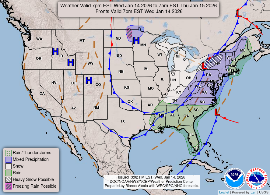 Weather Map
 Local Radar