6. LARGE SAMPLE EVALUATION OF TWO METHODS TO CORRECT RANGE DEPENDANT ERROR FOR WSR-88D RAINFALL ESTIMATESBertrand Vignal and Witold F. Krajewski Submitted to Corresponding author address: |
|||||||||||||||||||||||||||||||||||||||||||||||||||||||||||||||||||||||||||||||||||||||||||||||||||||||||||||||||||||
|
Abstract The vertical variability of reflectivity is an important source of error that affects a estimation of rainfall quantities by radar. This error can be reduced if the vertical profile of reflectivity (VPR) is known. Different methods are available to determine VPR based on volume scan radar data. We tested two such methods. The first method, used in the Swiss meteorological service, estimates a mean VPR directly from volumetric radar data collected close to the radar. The second method takes into account the spatial variability of reflectivity and relies on solving an inverse problem in determination of the profile. To test these methods we used two years worth of archive level II radar data from the WRS-88D located in Tulsa, Oklahoma, as well as the corresponding rain gauge observations from the Oklahoma Mesonet. The results obtained in comparing rain estimates from radar data corrected for the VPR influence with rain gauge observation show the benefits of the methods but also their limitations. The performance of the two methods is similar but the inverse method consistently provides better results. However, it requires substantially more computational resources for use in operational environment. 6.1 Introduction Different sources of error affect radar rainfall estimates. These sources of error are well-known (see, for example, Zawadzki 1982; Austin 1987; Joss and Waldvogel 1990; Smith et al. 1996). To derive accurate rainfall estimates from radar measurements for meteorological or hydrological applications, the sources of systematic errors, or biases, should be considered and errors corrected. In particular, one has to deal with the sources of range dependant bias. Evaluation of methods of reducing range dependent bias, which arises due to the vertical variability of the reflectivity profile, is the central theme of our paper. The inhomogeneous vertical structure of radar echoes is an important source of range dependant bias in rainfall estimation based on data collected by the WSR-88D (Weather Surveillance Radar 1988 Doppler) radars as has been documented by Smith et al. (1996) and Fulton et al. (1998). The vertical structure of radar echoes is related to phase changes of hydrometeors, and the evolution of their size and shape distribution. The sampling geometry of the radar beam (for WSR-88D it is nominally 0.5o for the base scan elevation angle and 1o for the 3dB-beamwidth) associated with this vertical structure of radar echoes lead to biases in radar rainfall estimates that are range dependant. To mitigate the effects of this source of error in WSR-88D rainfall estimates a corrective scheme is needed. A common approach to this problem, based on radar data only, consists of estimating a function describing the evolution versus altitude of the radar reflectivity: the VPR. This VPR is then used to extrapolate radar reflectivity data aloft to the ground level. The literature offers a number of procedures for VPR estimation. Andrieu and Creutin (1995) and Andrieu et al. (1995) solved the inverse problem of retrieving mean VPR at hourly interval from radar measurements recorded at two elevation angles using discrete inverse theory. Joss and Lee (1995) explored the case of VPR estimation in the difficult context of mountainous region. Mean VPR is deduced in real time from radar data recorded at 20 elevation angles within a radius of 70 km from the radar. Kitchen et al. (1994) proposed to retrieve an "idealized" VPR for each pixel of the radar domain using radar data, surface observation and infrared satellite data. Smyth and Illingworth (1998) proposed an extension of this work to explore the cases of more complex situations where convective cells are embedded into larger stratiform precipitation area. This procedure is based on the discrimination between stratiform and convective precipitations. The method proposed by Kitchen et al. (1994) is applied to correct echoes classified as stratiform, whereas a climatological based profile is used for echoes classified as convective rain. Vignal et al. (1999) proposed a generalization of the VPR retrieval procedure method proposed by Andrieu and Creutin (1995) to radar data recorded at many elevation angles. This generalization makes possible to identify VPRs locally, typically at a scale of 20 km by 20 km. For this study, we selected two different methods to correct the VPR influence: (1) mean VPR (MVPR), obtained from radar data collected close to the radar (e.g. within a range of 100 km); and (2) local VPR (LVPR), deduced from radar data for small regions using an inverse method. The MVPR, the principles of which are described by Joss and Lee (1995), allows taking into account the actual information provided by radar data. A version of this method is used operationally by the Swiss Meteorological Service. The LVPR, proposed by Vignal et al. (1999) allows taking into account the variations in space of the VPR. Both methods have been evaluated before. Joss and Lee (1995) showed the benefits of the MVPR method used operationally by the Swiss Meteorological Institute, for rainfall rate estimation. Vignal et al. (2000) conducted a limited (based on only nine rain events) comparison of these two methods in the context of the Swiss radar network. The study indicates that the LVPR method, by taking into account the variability in horizontal space of the VPRs, resulted in improved accuracy of rainfall estimates from radar compared to the MVPR method. In this paper we preset another evaluation of the two methods, this time based on a large sample of radar data collected by the Tulsa, Oklahoma WSR-88D, mainly during the warm season. We consider that due to the differences of the rainfall regime between Switzerland and Oklahoma, and different radar characteristics, including the scanning strategy, the results obtained earlier by Vignal et al. (2000) may not be easily transferable. Our large-sample study mimics an operational application, and as such, allows a comprehensive and rigorous evaluation of the benefits and limitations of each method. There are two elements in our study. First, we develop a validation methodology suitable for evaluation of the VPR correction methods, and second, we compare the benefits and limitations of each method using a variety of criteria. Our validation methodology uses two years worth of radar data from the WSR-88D located in Tulsa, Oklahoma, and an accompanying database of rain gauge observations used to evaluate the improvement of rain quantity estimates associated with the corrections. The choice of our test location is particularly challenging considering the varied precipitation regime over Oklahoma, dominated by mid-latitude convective systems, but with significant stratiform rainfall contributions. As a by-product of our study we obtained a climatological VPR for northeast Oklahoma. This paper is then organized as follows. We devote Section 2 to the problem formulation and the methods used for estimating the VPRs. In Section 3 we deal with the database and the implementation of the VPR estimation methods. In Section 4 we present the VPR variability, and in Section 5 we discuss an evaluation of the VPR correction methods. 6.2 Formulation of the problem and VPR estimation methods a. Formulation of the problem At each range, the radar measurement integrates the reflectivity over a section of the radar beam. A simplified expression of the radar measurement can be written as:
where is the reflectivity measured by the radar at the location x, a is the elevation angle, Z(x,h) is the radar reflectivity at location x and altitude h, H+ and H- represent respectively the upper and lower limit of the radar beam and f represents the partial integral of the power distribution of the radar beam at altitude h which depends on the beam width 0. The rainfall rate is deduced form the reflectivity through the use of a Z-R relationship. We assume that the function Z(x,h) can be factorized according to the following form: , (2) where Z(x,0) represents the radar reflectivity field at the ground level, the dimensionless factor is called the vertical profile of reflectivity (hereafter VPR). The VPR is assumed to be homogeneous within the geographic domain D and representative of the vertical variations of reflectivity in this domain. Relation (1) can be written: , (3) with , (4) where zDa is called the apparent vertical profile of reflectivity. It quantifies the difference between the reflectivity at ground level and the reflectivity measured by the radar at the point (x,a). Correcting the VPR influence can be easily achieved using (4) if the VPR is known. A correction factor is applied multiplicatively to each radar measurement. Considering rain rate measurement (rainfall rate deduced from the reflectivity through the use of a Z-R relationship), this correction factor is expressed: , (5) where P(x,a) is the correction factor to be applied to the rain rate measured by the radar at location x and b is the exponent of the Z-R relationship. The magnitude of this correction is illustrated by an example shown in Figure 1a. The VPR (Fig. 1b) has a reflectivity peak at an altitude of 2.0 km above which, the reflectivity decreases to -20 dB at an altitude of 6.5 km. This VPR is representative of a cold cloud leading to a marked bright band caused by the melting of ice particles. The correction factors versus range, related to this VPR, are shown in Figure 1a. We show two curves for the elevation angle of 0.5� and 1.5�. The beam width is 0=1� and the exponent b=1.4 (WSR-88D default Z-R relationship). For the 0.5� case, the correction factor is lower than 1 when the radar beam intersects the melting layer (between 70 and 160 km); without the correction radar rainfall estimates are overestimated. The correction factor is greater than 1 when the radar beam is above the melting layer (between 160 and 200 km), and without correction radar rainfall estimates are underestimated. b. Estimation of M VPR The mean apparent profile is directly obtained by averaging radar data collected within a 100 km radius at different altitudes. The range is restricted to 100 km to avoid the smoothing effects of the radar beam. In addition, in Switzerland this restriction is also motivated by problems of beam blocking. The mean profile is then used to correct the radar data over the whole radar domain. If not enough rain is recorded close to the radar, a climatological profile is used instead. Further details about this procedure, used operationally in Switzerland, can be found in Joss and Lee (1995). c. Estimation of LVPR In this section we briefly summarize the VPR identification algorithm proposed by Vignal et al. (1999). The initial version of this method, proposed by Andrieu and Creutin (1995), retrieves VPR from radar data recorded at two elevation angles. Vignal et al. (1999) generalized it to include data from more elevation angles available in voluminal radar scans. According to the method LVPRs are identified in areas of about 20 km by 20 km. Vignal et al. (1999) showed that these local profiles differ from the "true" ones because of the smoothing effect of the radar beam when the region of analysis is further than 50 km from the radar. It is inappropriate to correct radar data using such profiles. Clearly, a procedure for retrieval of the "true" profile is required. The main assumption of the method is that the VPR is homogeneous in the region of analysis, which permits separation of horizontal and vertical variations of the reflectivity (2). The ratio of two radar data, expressed in rainfall intensity, observed at a given location and at two different elevation angles can be written as follows: , (6) where is the intensity ratio measured at the distance x, a1 and ai are the elevation angles (a1 being the lowest one). The ratio allows filtering the horizontal variations of the radar reflectivity at ground, where the intensity ratio depends only on the radar beam and the VPR characteristics. In the region of analysis, by averaging these ratios over azimuth, average ratio versus distance is obtained. Considering the distance interval associated with the region of analysis, a ratio curve becomes a characteristic of the VPR. In Figure 2 we show an example of the set of ratio curves in a distance interval 40-60 km. We simulated these curves using the theoretical model (6) and an arbitrary VPR shown in Fig. 1b. Variations of ratios with distance are due to the increase of the beam height with range. Differences between two ratio curves are due to the different elevation angles considered. A set of ratio curves can be considered as the signature of the VPR in the region of analysis. The light shaded region corresponds to a range used in LVPR estimation. and the dark shaded region denotes the range where the 0.5� is not a good reference anymore as the radar beam intercepts the bright band. The objective of the identification method is to determine the VPR consistent with observed ratio curves. To perform this identification, different elements are available: i) the set of ratio curves, ii) the theoretical model (5) relating the ratios and the VPR, iii) the apparent VPR. The VPR identification consists of determining the VPR which leads through (5) as close as possible (in the sense of least square minimization) to the observed ratios curves. To solve this inverse problem (Menke, 1989) we used the algorithm proposed by Tarantola and Valette (1982a, b). We initialize this algorithm using the local apparent VPR directly deduced from voluminal radar data. For details see Andrieu and Creutin 1995 and Andrieu et al. 1995). Vignal et al (1999) showed that this procedure allows effective identification of the VPRs by range intervals. As a consequence, to apply this method, we divide the radar domain into several regions of analysis. For each region of analysis, we compute the ratio curves of radar data. We use these ratio curves to identify the local VPR. The LVPR is then used to correct the radar data for the given region. 3. The database and application conditions of the VPR estimation methods We test the effectiveness of correcting the range dependent errors in radar reflectivity using two years (1994 and 1995) of volumetric data from the WSR-88D Tulsa, Oklahoma, radar. First, the radar data were converted from the Archive Level II format (Klazura and Imy 1993) to the efficient format developed by Kruger and Krajewski (1997). To improve the quality of the data we applied the anomalous propagation echo detection method developed by Grecu and Krajewski (2000). We document the results in Krajewski and Vignal (2000). For the WSR-88D radars, the 3 dB beam width is 1� and the radar performs full volume scan every 6 minutes. Nominally, each volume scan is composed of nine scans at elevation angles increasing from 0.5� to 19.5� for a range of 200 km. We converted radar measurements (Z) into rainfall intensities (R) using the WSR-88D default relationship, Z=300R1.4. We also used the Oklahoma Mesonet (Brock et al. 1995) data to calculate hourly rainfall accumulations at 49 locations within the radar domain (Figure 3). Basic quality control for these data is carried out by the Oklahoma Climatological Survey (Shafer et al. 2000). The precipitation regime for the region is dominated by midlatitude convective systems (Houze et al. 1990; Houze 1993). To properly simulate an operational application of the procedure using mean apparent profile, a climatological VPR has to be estimated first. We estimated a climatological VPR using two years of the radar observed profiles and averaging them with weights being the mean rainfall intensity over the region of analysis (range of 100 km from the radar). This profile (Figure 4) displays a peak of reflectivity (+2.5 dB) at height of 2.8 km. This altitude can be interpreted as the mean level of the bright band. Above, the reflectivity decreases linearly with altitude at the rate of 2dB/km. Vignal et al (1999) performed an investigation of the appropriate conditions of LVPR identification. The study led to the following conclusions: i) VPR can be correctly identified by range intervals, ii) the accuracy decreases when the range interval is far from the radar, iii) the range interval must be increased with distance in order to retrieve the VPR with the same efficiency as for closer ranges. Following Vignal et al. (1999), we divided the radar domain into 144 regions of analysis as illustrated in Figure 5. Each region of analysis is 15� wide in azimuth and the radial extent increases with distance from the radar. For numerical reasons, we estimated discretized VPR with h=0.2 km step. For both methods, we estimated hourly VPRs. 6.4 The VPRs a. The MVPRs We obtained 410 MVPRs analyzing over 1000 hours of data. We show a subset of these in Figure 6. These VPRs exhibit a wide range of behavior. However, they have several features in common. First, the reflectivity is nearly constant in the lowest 2 km above the ground. Second, many of the VPRs display an enhancement of the reflectivity (up to 9.5 dB) at a certain height. Most of the time, it can be associated with the presence of stratiform precipitation. The altitude of this bright band differs from one VPR to another but typically is at about 2 km in March and 3.5 km in July. Third, at higher levels (above 4 km) the reflectivity decreases with increasing altitude. This decrease of the reflectivity varies from -7 dB/km to -1 dB/km. When a strong enhancement of the reflectivity is observed, the reflectivity decreases faster above 4 km than in absence of a strong enhancement. These VPRs explains qualitatively the bias observed between rainfall accumulation from radar and from rain gauges (see section 5). Considering rainfall accumulation deduced from radar data recorded at an elevation angle of 0.5�, no important bias is observed up to a distance of 100 km. For this range, the altitude of the beam axis is below 1.5 km. Between 100 km and 200 km, radar estimates are biased high. The altitude of the beam axis lies between 1.5 km to 4 km. If we consider rainfall accumulation deduced from radar data recorded at an elevation angle of 1.5�, no important bias is observed from the radar up to only 50 km (the altitude of the beam axis is above 1.5 km). Radar rainfall accumulations are overestimated from 50 km to about 120 km where the altitude of the beam axis is between 1.5 km and 4 km. At farther distance radar rainfall accumulations are underestimated. We have to recognize that these MVPRs only provide an incomplete perception of the variability of the VPRs. As a consequence, for example, these VPRs incorrectly represent cases where convective cells are embedded in larger stratiform precipitation regions. a. The LVPRs Locally identified VPRs provide better information on the variability in time and space of the VPRs. Figure 7 illustrates the variations in time and space of the VPR at the scale of a rain event. We show (Figure 7a) hourly accumulations estimated from the lowest PPI (elevation angle of 0.5�) for the event of May 8, 1995 at 03h LTC. High spatial variability of the rain amounts obtained for this hour over the radar domain is evident. This example is typical of the rainfall regime in Oklahoma where convective cells produce areas of high rain amount whereas large areas of more stratiform rain produce weaker rain amount. The associated VPRs obtained for this hour between ranges of 60 to 90 km are presented in Figure 7b. Two groups of VPRs can be distinguished. The first group (A) is typical for stratiform rain (strong bright band enhancement and fast decrease of the reflectivity above it). We notice than the VPRs taken at different locations are very similar to each other. The bright band is at an altitude of 2.8 km and is associated with an enhancement of +9dB. Above this bright band the decrease of the reflectivity with height is at the rate of about -4 dB/km. The second group of VPRs (B) is typical for convective cells and regions of transition between stratiform and convective rain. Some of these profiles are similar to the previous one, whereas others display no bright band and a weaker negative gradient (-3 dB/km). In general, we observe greater variability of VPR in this group. Let us compare these VPRs to those obtained at a single location over a period of time. The VPRs obtained between 60-90 km and 270�-285� in azimuth, from eleven hours of rain, are presented in Figure 7c. This set of VPRs is very similar to the one presented in Figure 7b. In Figure 8 we show the space-time variability of the LVPRs based on two years of data. The shown VPRs, obtained between 60 to 90 km, correspond to different accumulations of average area rainfall. For the VPRs shown in Figure 8a the averaged hourly accumulation is between 1.75 to 2.25 mm, while for the VPRs shown in Figure 8b, the averaged hourly accumulation is between 9.5 to 10.5 mm. For both cases we observe wide range of VPR behavior. When the mean hourly rainfall accumulation is increasing, we see a tendency of VPRs to decrease less with height. The averaged VPRs shown in Figures 8a and 8b illustrate this point. At the same time, the probability of bright band is greater for weak mean rainfall accumulation (35% of the profiles exhibits an enhancement greater the +3dB) than for larger mean rainfall accumulation (26% of the profiles exhibits an enhancement greater the +3dB). These observations reflect the fact that for weak mean rainfall accumulations, the VPRs are more typical for stratiform rain while larger accumulations correspond to convective conditions. However, it is only true on average. For low mean rainfall accumulation, weak decrease of the reflectivity with height without bright band enhancement can be observed, whereas for large mean rainfall accumulation, some profiles are characterized by a rapid decrease of the reflectivity with height and a localized strong enhancement of the reflectivity. 6.5 Evaluation of the two methods In this section we evaluate radar rainfall estimates considering (1) radar data only; and (2) radar-gauge comparison. In addition to considering radar rainfall estimates from radar data recorded at an elevation angle of 0.5� we also used 1.5� and 2.5�. This allows some generalization of our results for a situation where hybrid scans have to be constructed radar rainfall map. a. Evaluation using radar data only This evaluation is performed considering radar rainfall accumulation over the two years of data. Figures 9a, b and c show the uncorrected, corrected using the MVPR and corrected using the LVPR radar rainfall accumulation (in mm), respectively. Such long duration maps are useful in identifying range biases that cannot be detected if short duration maps are used due to large natural variability of rainfall. These figures show that, even considering two years of rainfall accumulation, natural variability of rainfall is important. A gradient of rain amount (from the northwest of the radar umbrella with the lower rain amounts to the southern one with higher rain amounts) is observed. A similar trend is evident considering rain amount from gauges. Also visible is partial beam blockage, especially in the northeastern part of the radar domain, see Fig. 9a. The impact of both VPR corrections is significant at range greater than 150 km in the southern part of the radar domain. Considering radar data recorded at higher elevation angles (1.5� and 2.5�) the impact of the VPR correction is more evident, the VPR influence being more important. To complete this analysis of total accumulation, let us consider azimuthally averaged radar rainfall accumulations (Figure 10). We assumed that the rainfall climatology does not depend on distance and thus, the range dependence of the mean radar-rainfall accumulations is induced by radar estimation error. Solid line in Fig. 10a is for rainfall accumulation from radar data recorded at 0.5� without VPR correction, dotted line is for radar data corrected using mean apparent VPRs and dashed line from data corrected using local identified VPRs. Fig. 10a, b and c, show rainfall accumulation form radar data recorded at 0.5�, 1.5� and 2.5�, respectively. At far range, the range dependence of mean radar rainfall accumulation is weak but significant. Both VPR correction procedures reduce this range dependence. Considering the higher elevation angles (Fig. 10b and c), the range dependence of mean radar rainfall accumulation is more important and so is the benefit of the VPR correction procedures. b. Evaluation using radar data and rain-gauge measurements In this and the following sub-sections we use rain gauge data are to assess the accuracy of the radar rainfall estimates and the improvement obtained using the different VPR correction method. Despite the conceptual problems associated with using rain gauges to evaluate radar estimates (Zawadzki 1982; Ciach and Krajewski 1999), we consider the differences between the collocated radar and gauge data as a viable performance measure. Our main interest is in hourly rainfall accumulation as justified by the needs of hydrological modeling for catchments of about 500 km2. We also consider daily rainfall accumulations and two-year totals. These larger integration times are of interest in climatological analyses. We compare rain gauge hourly observation with the radar rainfall accumulation estimate from the closest radar pixel on the polar grid. Figure 11 shows the scatter-plots of hourly rainfall accumulations stratified by the distance between the radar and the rain gauges. The three cases we show are for rainfall accumulations from radar data recorded at an elevation angle of 0.5�, (1) after mean apparent VPR based correction; (2) after locally identified VPR based correction; and (3) from radar data without VPR correction. We used the root mean square of the difference between radar and a collocated gauge (RMS) and the mean difference between radar and gauge (BIAS) to quantify the gain obtained using VPR correction procedure. The statistics are calculated based on hourly accumulations for those hours when both radar and rain gauge data are available. The results, stratified by range are shown in Table 1. Considering all the gauges, the mean apparent VPR based correction allows to reduce the RMS from 0.77 mm to 0.73 (reduction of 5%). The local identified VPR correction leads to reduce the RMS to 0.66 (reduction of 14%). The average hourly accumulation bias is 0.04 mm without VPR correction and is reduced to 0.01 mm with either of the VPR correction procedures. At this point we would like to point out that the RMS improvement we obtained underestimates the actual effect of the VPR schemes. This is because the radar and rain gauge difference are due to two combined effects: (1) the natural variability of rainfall in space; and (2) the radar-rainfall estimation error that includes numerous sources of uncertainty. This issue is thoroughly discussed by Ciach and Krajewski (1999). Following the Error Separation Method (ESM) they proposed, Young et al. (2000) attempted to estimate the uncertainty of the hourly rainfall product used by the Tulsa River Forecast Office of the National Weather Service, but concluded that they lack sufficient information about the small scale variability of rainfall. Since our study uses similar rain gauge data set, we do not attempt relevant analysis. Therefore, our estimate of RMS error improvement is conservative by as much as 50% if the natural rainfall variability is significant. The benefits of the VPR correction procedures are more obvious if we consider a reduction of the range dependence of the values of RMS and BIAS. Without VPR correction, the values of RMS (BIAS) are between 0.63 (-0.02) considering gauges between 50 to 100 km from the radar to 0.91 mm (0.08 mm) considering gauges between 150 to 200 km from the radar. Thus, close to the radar, the VPR does not affect much the radar estimates. At far ranges (greater than 100 km), because of the VPR influence, radar-rainfall values are often overestimated (see Fig. 11). The overestimation can be related to the bright band influence. Considering mean apparent VPR based correction, the range dependence of the RMS is reduced only until 150 km whereas the BIAS is reduced for all ranges. The values of RMS (BIAS) are between 0.62 mm (-0.03 mm) for gauges between 50 to 100 km from the radar to 0.69 mm (0.01 mm) for gauges between 100 to 150 km from the radar. Between 150 and 200 km the MVPR based corrections only marginally improve the accuracy of radar rainfall estimates in term of RMS. This result comes from inaccurate corrections for some particular hours (see Fig. 11). At these distances, the MVPRs can induce large correction. When these corrections are inaccurate, because for example, of a lack of representativity of the VPR, a large error is introduced. Considering LVPR based corrections, the values of RMS (BIAS) are between 0.62 mm (-0.03 mm) for gauges between 50 to 100 km from the radar to 0.74 mm (0.01 mm) for gauges between 150 to 200 km from the radar. Considering the gauges closed to the radar (up to 100 km), the VPR correction impact (Fig. 11) is weak. Far from the radar, the impact is more significant. We also computed the values of RMS and BIAS for daily and total rainfall accumulations (see Table 1). For daily accumulation, the gain achieved using VPR based correction is more important. The RMS is 3.85 mm without VPR correction, 3.31 mm (14% reduction) considering mean apparent VPR correction and 2.89 mm (25% reduction) considering LVPR correction. With larger time scales of accumulation, problems of representativeness of gauges we alluded to above are less significant. Similarly, are problems related to the choice of the Z-R relationship. The larger time scales also reduce the effect of punctually inaccurate VPR correction. The benefit of using LVPR instead of mean apparent VPR is smaller than for hourly accumulations. The values of RMS obtained considering total accumulation confirm this. The RMS is 75 mm without VPR correction, 51 mm (32% reduction) considering MVPR correction and 44 mm (41% reduction) considering LVPR correction. In this case the benefit of using LVPR instead of MVPR appears to be marginal. We also evaluated radar rainfall estimates deduced from radar data recorded at higher elevation angles (1.5� and 2.5�). Our motivation was to study the situation when due to total or partial occultation of the lowest beam, higher elevation data must be used. This is often the case in mountainous regions. As the VPR is more influential at higher elevation angles, the benefit of using a VPR correction should be more substantial. The results are shown in Table 2. For the radar data recorded at an elevation angle of 1.5�, the agreement between radar and gauge is weaker than considering radar data recorded at 0.5�. Between 0 to 100 km from the radar, radar data can be affected by the bright band influence (BIAS greater than 0 mm). At distance greater than 100 km, most of the time, the radar beam is above the melting layer (BIAS lower than 0 mm). Without any correction, the RMS is 1.06 mm (against 0.77 mm for radar data at 0.5�). The VPR correction procedure reduces the values of RMS: 0.87 mm for the MVPR based procedure and 0.80 mm for the LVPR based procedure. Weaker agreements than for 0.5� are obtained. This result reflects the limitations of the VPR correction procedures at far range (over 150 km considering this elevation angle). These limitation are due to i) beam overshooting (no possible correction when the radar beam is above the echo top) and ii) a better correlation between surface rainfalls with water-coated frozen hydrometeors in the melting layer than with ice particles well above the freezing level (Seo and Breidenbach, 1998). As a consequence, after VPR correction radar data recorded at 1.5� provide "accurate" rainfall estimates only up to about 150 km. Considering radar data recorded at 2.5�, this range is further restricted to about 100 km. b. Seasonal analysis To better investigate the benefits and limitations of the VPR correction procedures we performed a seasonal analysis. We divided data into a warm season (May to October), dominated by convective rainfall, and a cold season (November to April), dominated by widespread stratiform precipitation. Smith et al. (1996) proposed, for the same location, an extended warm season (from April to October). Considering our data and looking at the vertical structure of radar echoes, we find that April 1994 and 1995 were dominated by widespread stratiform precipitation. Based on this observation, we included April into the cold season. One can expect a more important-but easier to correct-influence of the VPR for the cold season than for the warm season. The results of the comparison between radar and gauge, for both seasons, are presented in Table 2. For the cold season, both VPR estimation procedures allow reducing the difference between radar and gauge. The RMS (BIAS) is 0.87 mm (0.08) without VPR correction, 0.76 (0.02) using the MVPR based procedure (reduction of 13% of the RMS) and 0.68 (0.01) using the LVPR based procedure (reduction of 22% of the RMS). For the cold season, the MVPR based procedure reduces the difference between radar and gauge as far as 200 km from the radar, although the improvement is insignificant beyond 150 km. For the warm season, only the LVPR based procedure allows reducing the difference between radar and gauge in term of RMS and both methods in term of BIAS. The RMS (BIAS) is 0.69 mm (0.01 mm) without VPR correction, 0.70 (0.01 mm) using the MVPR based procedure and 0.65 (0.01 mm) using locally identified VPR. These results show that it is more difficult to correct for the VPR influence for the warm season. In particular, the MVPR based procedure increases (in term of RMS) the difference between radar and gauge at distance greater than 100 km from the radar. 6. Conclusions and outlook We described an evaluation of two methods of correcting the vertical profile of reflectivity in WSR-88D radar data and the corresponding improvements in rainfall estimates. Using two years of data from the WSR-88D in Tulsa, Oklahoma, and the Oklahoma Mesonet rain gauge database, we compared the two methods according to several criteria applied at various temporal scales of integration. The first method to determine the VPR is similar to the one used operationally in Switzerland and provides mean apparent VPR obtained from data at close ranges. The second method provides locally identified VPR for areas of about 20 km by 20 km. As the VPR induces range dependant errors in long-term accumulation of rainfall, both correction methods contribute to reducing them. We found slightly better results using the locally identified VPR. Both methods reduce significantly the bias between radar and gauge daily and hourly rainfall estimates. Both also reduce the RMS error but here the performance of the locally identified VPR is much better. The difference between the two methods, however, decreases as the time scale increases. We also found that the VPR is more influent and a correction more effective during the cold season and for lower rainfall intensities than for the warm season and larger rainfall intensities. Finally, we briefly investigated the influence of the natural variability of rainfall on our comparison between radar and gauge. As we lack adequate information on small scale rainfall variability we did not perform a comprehensive investigation. However, since the effect of natural variability is range dependent (as the radar averaging area increases with distance from radar) it interfered with our results. This influence of the natural variability of rainfall has to be accounted to obtain a representative influence of the VPR corrections. As a by-product of the study, we obtained a VPR climatology. This VPR climatology can be used for radar rainfall error parameterization or error evaluation purposes. Another potential application is related to short-term rainfall forecasting methods. Some of the models used require estimates of the vertically integrated rainwater content (VIL) which can be deduced from the VPRs (see, for instance, French and Krajewski, 1994). Based on our study we conclude that both investigated methods have serious shortcoming as far as being considered for operational real time application. Mean apparent VPRs method can lead to large inappropriate corrections. Locally identified VPRs method is very expensive in term of computer memory allocation (3 times more than the other method) and time computer consuming (about 10 times more). A compromise method, specifically dedicated to WSR-88D rainfall estimates and proposed by Seo et al. (2000), takes into account the smoothing effect of beam widening and is computationally efficient. A long-term evaluation of this method is currently under investigation, and we will report results in the near future. Still, the method does not take into account the geographical variability of the VPR as the LVPRs do. One way to partially deal with this problem is to define criteria to apply or not the corrections associated to the mean VPR based on some sort of classification of the radar echoes (e.g. stratiform versus convective, see Steiner et al. 1995) and to estimate independently the associated VPRs. The idea is to capture the main geographical variations of the VPR. We also need to point out that we did not use optimized algorithms for rainfall estimation. Optimal setting of Z-R relationship as well as other parameters, along with a pre-classification of rainfall should further improve the reported results. Acknowledgements: This study was supported under the Cooperative Agreement between the Office of Hydrology of the National Weather Service (NWS) and the Iowa Institute of Hydraulic Research (NA47WH0495). We thank Dong Jun Seo of NWS for many valuable comments in the course of this study. References
Table 1: Root mean square (and bias) of the difference between hourly, daily and total accumulations from radar and gauge reflecting the improvement of rain estimates considering the two profile corrections and, for reference, without VPR correction. Table 2: Root Mean Square (and bias) of the difference between hourly rainfall accumulation from radar data (recorded at 0.5�, 1.5� and 2.5� of elevation angle) and gauge. Table 3: Root Mean Square (and bias) of the difference between hourly rainfall accumulation from radar data and gauge considering a warm and a cold season. Figure 1. Illustration of VPR correction curves for two elevation angles (panel A) associated with an arbitrary vertical profile of reflectivity VPR (panel B). Figure 2. Example of ratio curves of radar data simulated using the VPR shown in Fig. 1b. The light shaded region corresponds to one 20 km interval used in LVPR correction calculations. The dark shaded region denotes distance over which no VPR corrections should be made as the lowest angle (0.5�) is not a good reference anymore. Figure 3. Locations of the Oklahoma Mesonetwork rain gauges used in this study (circles ndicate 50, 100, 150 and 200 km range from radar site). Only Oklahoma part of the radar mbrella is shown. Figure 4. Regions of analysis used to estimate locally identified VPRs. Figure 5. Two-year sample of the MVPRs and the climatological VPR (thick line). Figure 6. Illustration of the variability in time and space of the LVPRs. (A) Hourly mean rain-rate from radar data recorded at 0.5� (05/08/95 at 03:00 a.m.), also shown are 24 sectors are selected for illustrating the variability in space of the VPR. (B) Corresponding LVPRs, divided into two groups (group a corresponds to area of stratiform rain, group b corresponds to convective rain as marked in A). (C) Time series of the VPRs obtained over the bold-marked sector divided into two groups according to time during the same storm. Figure 7. Conditional sample of locally identified VPRs obtained between 60-90 km from the radar. (A) VPR obtained on region of analysis where radar data at 0.5� reported an average rainfall between 0.75 to 1.25 mm/h. (B) VPR obtained on region of analysis where radar data at 0.5� reported an average rainfall between 9.50 to 10.50 mm/h. Figure 8. Two-year accumulation map based on radar data recorded at an elevation of 0.5� (A) without VPR correction; (B) corrected using MVPR; and (C) corrected using LVPR. Figure 9. Azimuthally averaged two-year accumulation based on radar data recorded at (A) 0.5�; (B) 1.5�; and (C) 2.5�. Continuous lines are for radar data without VPR correction, dotted lines for radar data corrected using MVPRs and mixed lines for radar data corrected using LVPR. Figure 10. Comparisons of hourly accumulations based on gauges versus radar organized by distance from the radar. Figure 11. Gauge by gauge analysis of mean hourly bias as a function of the distance from the radar: (A) mean hourly accumulation from gauges; (B) mean hourly bias between gauge and radar without VPR correction; (C) between gauge and radar corrected using MVPR; and (D) corrected using LVPR. Figure 12. Bias between radar and gauge total rainfall accumulation, for radar data (A) before QC; (B) after QC; (C), after QC and MVPR correction; and (D) after QC and LVPR correction. Table 1: Root Mean Square (and bias) of the difference between hourly, daily and total accumulations from radar and gauge reflecting the improvement of rain estimates considering the two profile corrections and, for reference, without VPR correction.
Table 2: Root Mean Square (and bias) of the difference between hourly rainfall accumulation from radar data (recorded at 0.5�, 1.5� and 2.5� of elevation angle) and gauge.
Table 3: Root Mean Square (and bias) of the difference between hourly rainfall accumulation from radar data and gauge considering a warm and a cold season.
Figure 1. Illustration of VPR correction curves for two elevation angles (panel A) associated with an arbitrary vertical profile of reflectivity VPR (panel B). 
Figure 2. Example of ratio curves of radar data simulated using the VPR shown in Fig. 1B. The light shaded region corresponds to one 20 km interval used in LVPR correction calculations.The dark shaded region denotes distance over which no VPR corrections should be made as the lowest angle (0.5�) is not a good reference anymore. 
Figure 3. Locations of the Oklahoma Mesonetwork rain gauges used in this study (circles indicate 100 and 200 km range from radar site). Only Oklahoma part of the radar umbrella is shown. 
Figure 4. Regions of analysis used to estimate locally identified VPRs. 
Figure 5. Two-year sample of the MVPRs and the climatological VPR (thick line).  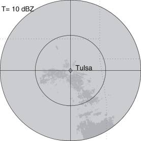 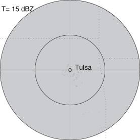 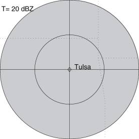
Figure 6. Illustration of the variability in time and space of the LVPRs. (A) Hourly mean rain-rate from radar data recorded at 0.5� (05/08/95 at 03:00 a.m.), also shown are 24 sectors are selected for illustrating the variability in space of the VPR. (B) Corresponding LVPRs, divided into two groups (group a corresponds to area of stratiform rain, group b corresponds to convective rain as marked in A). (C) Time series of the VPRs obtained over the bold-marked sector divided into two groups according to time during the same storm. 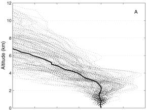 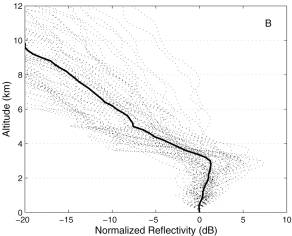 Figure 7. Conditional sample of locally identified VPRs obtained between 60-90 km from the radar. (A) VPR obtained on region of analysis where radar data at 0.5� reported an average rainfall between 0.75 to 1.25 mm/h. (B) VPR obtained on region of analysis where radar data at 0.5� reported an average rainfall between 9.50 to 10.50 mm/h. 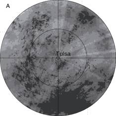 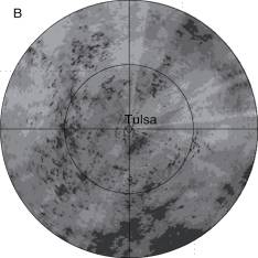 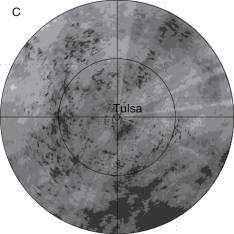 
Figure 8. Two-year accumulation map based on radar data recorded at an elevation of 0.5� (A) without VPR correction; (B) corrected using MVPR; and (C) corrected using LVPR. 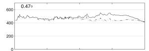 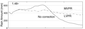 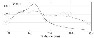
Figure 9. Azimuthally averaged two-year accumulation based on radar data recorded at (A) 0.5�; (B) 1.5�; and (C) 2.5�. Continuous lines are for radar data without VPR correction, dotted lines for radar data corrected using MVPRs and mixed lines for radar data corrected using LVPR. 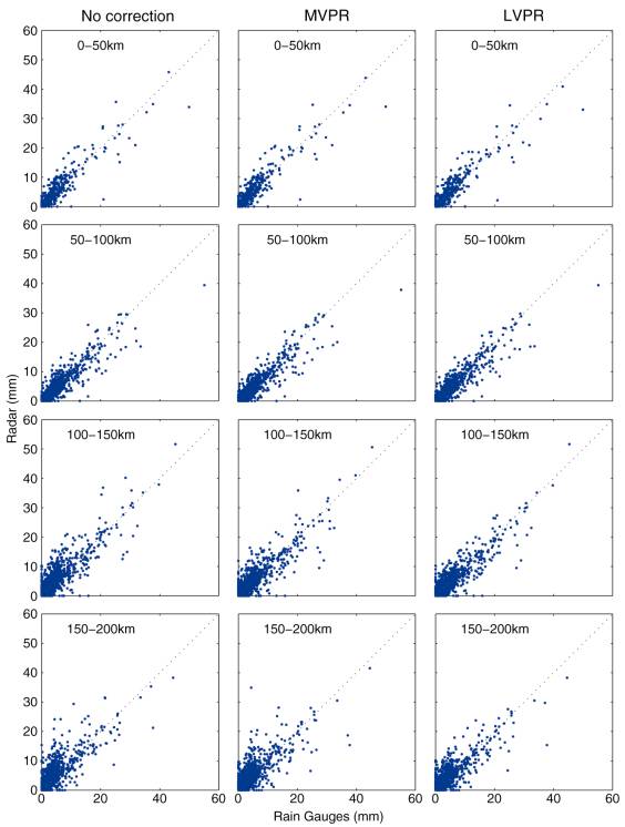
Figure 10. Comparisons of hourly accumulations based on gauges versus radar organized by distance from the radar. 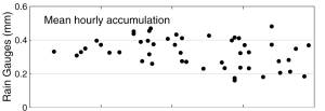 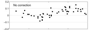 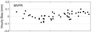 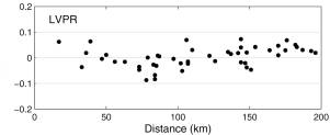
Figure 11. Gauge by gauge analysis of mean hourly bias as a function of the distance from the radar: (A) mean hourly accumulation from gauges; (B) mean hourly bias between gauge and radar without VPR correction; (C) between gauge and radar corrected using MVPR; and (D) corrected using LVPR.
Figure 12. Bias between radar and gauge total rainfall accumulation, for radar data (A) before QC; (B) after QC; (C), after QC and MVPR correction; and (D) after QC and LVPR correction. |
|||||||||||||||||||||||||||||||||||||||||||||||||||||||||||||||||||||||||||||||||||||||||||||||||||||||||||||||||||||
|
Main Link Categories: Home | OHD | NWS |